Table of Contents
Introduction
I recently wrote a big two-part series about a ton of things that I learned throughout the process of porting my hobby renderer, Takua Renderer, to 64-bit ARM.
In the second part, one of the topics I covered was how the Embree ray tracing kernels library gained arm64 support by utilizing the sse2neon project to emulate x86-64 SSE2 SIMD instructions using arm64’s Neon SIMD instructions.
In the second part of the series, I had originally planned on diving much deeper into comparing writing vectorized code using SSE intrinsics versus using Neon intrinsics versus other approaches, but the comparison write-up became so large that I wound up leaving it out of the original post with the intention of making the comparison into its own standalone post.
This post is that standalone comparison!
As discussed in my porting to arm64 series, a huge proportion of the raw compute power in modern CPUs is located in vector SIMD instruction set extensions, and lots of things in computer graphics happen to be be workload types that fit vectorization very well.
Long-time readers of this blog probably already know what SIMD instructions do, but for the unfamiliar, here’s a very brief summary.
SIMD stands for single instruction, multiple data, and is a type of parallel programming that exploits data level parallelism instead of concurrency.
What the above means is that, unlike multithreading, in which multiple different streams of instructions simultaneously execute on different cores over different pieces of data, in a SIMD program, a single instruction stream executes simultaneously over different pieces of data.
For example, a 4-wide SIMD multiplication instruction would simultaneously execute a single multiply instruction over four pairs of numbers; each pair is multiplied together at the same time as the other pairs.
SIMD processing makes processors more powerful by allowing the processor to process more data within the same clock cycle; many modern CPUs implement SIMD extensions to their base scalar instruction sets, and modern GPUs are at a very high level broadly similar to huge ultra-wide SIMD processors.
Multiple approaches exist today for writing vectorized code.
The four main ways available today are: directly write code using SIMD assembly instructions, write code using compiler-provided vector intrinsics, write normal scalar code and rely on compiler auto-vectorization to emit vectorized assembly, or write code using ISPC: the Intel SPMD Program Compiler.
Choosing which approach to use for a given project requires considering many different tradeoffs and factors, such as ease of programming, performance, and portability.
Since this post is looking at comparing SSE2 and Neon, portability is especially interesting here.
Auto-vectorization and ISPC are the most easily portable approaches, while vector intrinsics can be made portable using sse2neon, but each of these approaches requires different trade-offs in other areas.
In this post, I’ll compare vectorizing the same snippet of code using several different approaches.
On x86-64, I’ll compare implementations using SSE intrinsics, using auto-vectorization, and using ISPC emitting SSE assembly.
On arm64, I’ll compare implementations using Neon intrinsics, using SSE intrinsics emulated on arm64 using sse2neon, using auto-vectorization, and using ISPC emitting Neon assembly.
I’ll also evaluate how each approach does in balancing portability, ease-of-use, and performance.
4-wide Ray Bounding Box Intersection
For my comparisons, I wanted to use a small but practical real-world example.
I wanted something small since I wanted to be able to look at the assembly output directly, and keeping things smaller makes the assembly output easier to read all at once.
However, I also wanted something real-world to make sure that whatever I learned wasn’t just the result of a contrived artificial example.
The comparison that I picked is a common operation inside of ray tracing: 4-wide ray bounding box intersection.
By 4-wide, I mean intersecting the same ray against four bounding boxes at the same time.
Ray bounding box intersection tests are a fundamental operation in BVH traversal, and typically account for a large proportion (often a majority) of the computational cost in ray intersection against the scene.
Before we dive into code, here’s some background on BVH traversal and the role that 4-wide ray bounding box intersection plays in modern ray tracing implementations.
Acceleration structures are a critical component of ray tracing; tree-based acceleration structures convert tracing a ray against a scene from being a O(N) problem into a O(log(N)) problem, where N is the number of objects that are in the scene.
For scenes with lots of objects and for objects made up of lots of primitives, lowering the worst-case complexity of ray intersection from linear to logarithmic is what makes the difference between ray tracing being impractical and practical.
From roughly the late 90s through to the early 2010s, a number of different groups across the graphics field put an enormous amount of research and effort into establishing the best possible acceleration structures.
Early on, the broad general consensus was that KD-trees were the most efficient acceleration structure for ray intersection performance, while BVHs were known to be faster to build than KD-trees but less performant at actual ray intersection.
However, advancements over time improved BVH ray intersection performance [Stich et al. 2009] to the point where today, BVHs are now the dominant acceleration structure used in pretty much every production ray tracing solution.
For a history and detailed survey of BVH research over the past twenty-odd years, please refer to Meister et al. [2021].
One interesting thing to note when looking through the past twenty years of ray tracing acceleration research are the author names; many of these authors are the same people that went on to create the modern underpinnings of Embree, Optix, and the ray acceleration hardware found in NVIDIA’s RTX GPUs.
A BVH is a tree structure where bounding boxes are placed over all of the objects that need to be intersected, and then these bounding boxes are grouped into (hopefully) spatially local groups.
Each group is then enclosed in another bounding box, and these boxes are grouped again, and so on and so forth until a top-level bounding box is reached that contains everything below.
In university courses, BVHs are traditionally taught as being binary trees, meaning that each node within the tree structure bounds two children nodes.
Binary BVHs are the simplest possible BVH to build and implement, hence why they’re usually the standard version taught in schools.
However, the actual branching factor at each BVH node doesn’t have to be binary; the branching factor can be any integer number greater than 2.
BVHs with 4 and even 8 wide branching factors have largely come to dominate production usage today.
The reason production BVHs today tend to have wide branching factors originates in the need to vectorize BVH traversal in order to utilize the maximum possible performance of SIMD-enabled CPUs.
Early attempts at vectorizing BVH traversal centered around tracing groups, or packets, of multiple rays through a BVH together; packet tracing allows for simultaneously intersecting N rays against a single bounding box at each node in the hierarchy [Wald et al. 2001], where N is the vector width.
However, packet tracing only really works well for groups of rays that are all going in largely the same direction from largely the same origin; for incoherent rays, divergence in the traversal path each incoherent ray needs to take through the BVH destroys the efficacy of vectorized packet traversal.
To solve this problem, several papers concurrently proposed a different solution to vectorizing BVH traversal [Wald et al. 2008, Ernst and Greiner 2008, Dammertz et al. 2008]: instead of simultaneously intersecting N rays against a single bounding box, this new solution simultaneously intersects a single ray against N bounding boxes.
Since the most common SIMD implementations are at least 4 lanes wide, BVH implementations that want to take maximum advantage of SIMD hardware also need to be able to present four bounding boxes at a time for vectorized ray intersection, hence the move from a splitting factor of 2 to a splitting factor of 4 or even wider.
In addition to being more performant when vectorized, a 4-wide splitting factor also tends to reduce the depth and therefore memory footprint of BVHs, and 4-wide BVHs have also been demonstrated to be able to outperform 2-wide BVHs even without vectorization [Vegdahl 2017].
Vectorized 4-wide BVH traversal can also be combined with the previous packet approach to yield even better performance for coherent rays [Tsakok 2009].
All of the above factors combined are why BVHs with wider branching factors are more popularly used today on the CPU; for example, the widely used Embree library [Wald et al. 2014] offers 4-wide as the minimum supported split factor, and supports even wider split factors when vectorizing using wider AVX instructions.
On the GPU, the story is similar, although a little bit more complex since the GPU’s SIMT (as opposed to SIMD) parallelism model changes the relative importance of being able to simultaneously intersect one ray against multiple boxes.
GPU ray tracing systems today use a variety of different split factors; AMD’s RDNA2-based GPUs implement hardware acceleration for a 4-wide BVH [AMD 2020].
NVIDIA does not publicly disclose what split factor their RTX GPUs assume in hardware, since their various APIs for accessing the ray tracing hardware are designed to allow for changing out for different, better future techniques under the hood without modification to client applications.
However, we can guess that support for multiple different splitting factors seems likely given that Optix 7 uses different splitting factors depending on whether an application wants to prioritize BVH construction speed or BVH traversal speed [NVIDIA 2021].
While not explicitly disclosed, as of writing, we can reasonable guess based off of what Optix 6.x implemented that Optix 7’s fast construction mode implements a TRBVH [Karras and Aila 2013], which is a binary BVH, and that Optix 7’s performance-optimized mode implements a 8-wide BVH with compression [Ylitie et al. 2017].
Since the most common splitting factor in production CPU cases in a 4-wide split, and since SSE and Neon are both 4-wide vector instruction sets, I think the core simultaneous single-ray-4-box intersection test is a perfect example case to look at!
To start off, we need an efficient intersection test between a single ray and a single axis-aligned bounding box.
I’ll be using the commonly utilized solution by Williams et al. [2005]; improved techniques with better precision [Ize 2013] and more generalized flexibility [Majercik 2018] do exist, but I’ll stick with the original Williams approach in this post to keep things simple.
Test Program Setup
Everything in this post is implemented in a small test program that I have put in an open Github repository, licensed under the Apache-2.0 License.
Feel free to clone the repository for yourself to follow along using or to play with!
To build and run the test program yourself, you will need a version of CMake that has ISPC support (so, CMake 3.19 or newer), a modern C++ compiler with support for C++17, and a version of ISPC that supports Neon output for arm64 (so, ISPC v1.16.1 or newer); further instructions for building and running the test program is included in the repository’s README.md file.
The test program compiles and runs on both x86-64 and arm64; on each processor architecture, the appropriate implementations for each processor architecture are automatically chosen for compilation.
The test program runs each single-ray-4-box intersection test implementation N times, where N is an integer that can be set by the user as the first input argument to the program.
By default, and for all results in this post, N is set to 100000 runs.
The four bounding boxes that the intersection tests run against are hardcoded into the test program’s main function and are reused for all N runs.
Since the bounding boxes are hardcoded, I had to take some care to make sure that the compiler wasn’t going to pull any optimization shenanigans and not actually run all N runs.
To make sure of the above, the test program is compiled in two separate pieces: all of the actual ray-bounding-box intersection functions are compiled into a static library using -O3 optimization, and then the test program’s main function is compiled separately with all optimizations disabled, and then the intersection functions static library is linked in.
Ideally I would have liked to set up the project to compile directly to a Universal Binary on macOS, but unfortunately CMake’s built-in infrastructure for compiling multi-architecture binaries doesn’t really work with ISPC at the moment, and I was too lazy to manually set up custom CMake scripts to invoke ISPC multiple times (once for each target architecture) and call the macOS lipo tool; I just compiled and ran the test program separately on an x86-64 Mac and on an arm64 Mac.
However, on both the x86-64 and arm64 systems, I used the same operating system and compilers.
For all of the results in this post, I’m running on macOS 11.5.2 and I’m compiling using Apple Clang v12.0.5 (which comes with Xcode 12.5.1) for C++ code and ISPC v1.16.1 for ISPC code.
For the rest of the post, I’ll include results for each implementation in the section discussing that implementation, and then include all results together in a results section at the end.
All results were generated by running on a 2019 16 inch MacBook Pro with a Intel Core i7-9750H CPU for x86-64, and on a 2020 M1 Mac Mini for arm64 and Rosetta 2.
All results were generated by running the test program with 100000 runs per implementation, and I averaged results across 5 runs of the test program after throwing out the highest and lowest result for each implementation to discard outliers.
The timings reported for each implementation are the average across 100000 runs.
Defining Structs Usable with Both SSE and Neon
Before we dive into the ray-box intersection implementations, I need to introduce and describe the handful of simple structs that the test program uses.
The most widely used struct in the test program is FVec4, which defines a 4-dimensional float vector by simply wrapping around four floats.
FVec4 has one important trick: FVec4 uses a union to accomplish type punning, which allows us to access the four floats in FVec4 either as separate individual floats, or as a single __m128 when using SSE or a single float32x4_t when using Neon.
__m128 on SSE and float32x4_t on Neon serve the same purpose; since SSE and Neon use 128-bit wide registers with four 32-bit “lanes” per register, intrinsics implementations for SSE and Neon need a 128-bit data type that maps directly to the vector register when compiled.
The SSE intrinsics implementation defined in <xmmintrin.h> uses __m128 as its single generic 128-bit data type, whereas the Neon intrinsics implementation defined in <arm_neon.h> defines separate 128-bit types depending on what is being stored.
For example, Neon intrinsics use float32x4 as its 128-bit data type for four 32-bit floats, and uses uint32x4 as its 128-bit data type for four 32-bit unsigned integers, and so on.
Each 32-bit component in a 128-bit vector register is often known as a lane.
The process of populating each of the lanes in a 128-bit vector type is sometimes referred to as a gather operation, and the process of pulling 32-bit values out of the 128-bit vector type is sometimes referred to as a scatter operation; the FVec4 struct’s type punning makes gather and scatter operations nice and easy to do.
One of the comparisons that the test program does on arm64 machines is between an implementation using native Neon intrinsics, and an implementation written using SSE intrinsics that are emulated with Neon intrinsics under the hood on arm64 via the sse2neon project.
Since for this test program, SSE intrinsics are available on both x86-64 (natively) and on arm64 (through sse2neon), we don’t need to wrap the __m128 member of the union in any #ifdefs.
We do need to #ifdef out the Neon implementation on x86-64 though, hence the check for #if defined(__aarch64__).
Putting everything above all together, we can get a nice, convenient 4-dimensional float vector in which we can access each component individually and access the entire contents of the vector as a single intrinsics-friendly 128-bit data type on both SSE and Neon:
struct FVec4 {
    union {  // Use union for type punning __m128 and float32x4_t
        __m128 m128;
#if defined(__aarch64__)
        float32x4_t f32x4;
#endif
        struct {
            float x;
            float y;
            float z;
            float w;
        };
        float data[4];
    };

    FVec4() : x(0.0f), y(0.0f), z(0.0f), w(0.0f) {}
#if defined(__x86_64__)
    FVec4(__m128 f4) : m128(f4) {}
#elif defined(__aarch64__)
    FVec4(float32x4_t f4) : f32x4(f4) {}
#endif

    FVec4(float x_, float y_, float z_, float w_) : x(x_), y(y_), z(z_), w(w_) {}
    FVec4(float x_, float y_, float z_) : x(x_), y(y_), z(z_), w(0.0f) {}

    float operator[](int i) const { return data[i]; }
    float& operator[](int i) { return data[i]; }
};
Listing 1: FVec4 definition, which defines a 4-dimensional float vector that can be accessed as either a single 128-bit vector value or as individual 32-bit floats.
The actual implementation in the test project has a few more functions defined as part of FVec4 to provide basic arithmetic operators.
In the test project, I also define IVec4, which is a simple 4-dimensional integer vector type that is useful for storing multiple indices together.
Rays are represented as a simple struct containing just two FVec4s and two floats; the two FVec4s store the ray’s direction and origin, and the two floats store the ray’s tMin and tMax values.
For representing bounding boxes, the test project has two different structs.
The first is BBox, which defines a single axis-aligned bounding box for purely scalar use.
Since BBox is only used for scalar code, it just contains normal floats and doesn’t have any vector data types at all inside:
struct BBox {
    union {
        float corners[6];        // indexed as [minX minY minZ maxX maxY maxZ]
        float cornersAlt[2][3];  // indexed as corner[minOrMax][XYZ]
    };

    BBox(const FVec4& minCorner, const FVec4& maxCorner) {
        cornersAlt[0][0] = fmin(minCorner.x, maxCorner.x);
        cornersAlt[0][1] = fmin(minCorner.y, maxCorner.y);
        cornersAlt[0][2] = fmin(minCorner.z, maxCorner.z);
        cornersAlt[1][0] = fmax(minCorner.x, maxCorner.x);
        cornersAlt[1][1] = fmax(minCorner.y, maxCorner.y);
        cornersAlt[1][2] = fmax(minCorner.x, maxCorner.x);
    }

    FVec4 minCorner() const { return FVec4(corners[0], corners[1], corners[2]); }

    FVec4 maxCorner() const { return FVec4(corners[3], corners[4], corners[5]); }
};
Listing 2: Struct holding a single bounding-box.
The second bounding box struct is BBox4, which stores four axis-aligned bounding boxes together.
BBox4 internally uses FVec4s in a union with two different arrays of regular floats to allow for vectorized operation and individual access to each component of each corner of each box.
The internal layout of BBox4 is not as simple as just storing four BBox structs; I’ll discuss how the internal layout of BBox4 works a little bit later in this post.
Williams et al. 2005 Ray-Box Intersection Test: Scalar Implementations
Now that we have all of the data structures that we’ll need, we can dive into the actual implementations.
The first implementation is the reference scalar version of ray-box intersection.
The implementation below is pretty close to being copy-pasted straight out of the Williams et al. 2005 paper, albeit with some minor changes to use our previously defined data structures:
bool rayBBoxIntersectScalar(const Ray& ray, const BBox& bbox, float& tMin, float& tMax) {
    FVec4 rdir = 1.0f / ray.direction;
    int sign[3];
    sign[0] = (rdir.x < 0);
    sign[1] = (rdir.y < 0);
    sign[2] = (rdir.z < 0);

    float tyMin, tyMax, tzMin, tzMax;
    tMin = (bbox.cornersAlt[sign[0]][0] - ray.origin.x) * rdir.x;
    tMax = (bbox.cornersAlt[1 - sign[0]][0] - ray.origin.x) * rdir.x;
    tyMin = (bbox.cornersAlt[sign[1]][1] - ray.origin.y) * rdir.y;
    tyMax = (bbox.cornersAlt[1 - sign[1]][1] - ray.origin.y) * rdir.y;
    if ((tMin > tyMax) || (tyMin > tMax)) {
        return false;
    }
    if (tyMin > tMin) {
        tMin = tyMin;
    }
    if (tyMax < tMax) {
        tMax = tyMax;
    }
    tzMin = (bbox.cornersAlt[sign[2]][2] - ray.origin.z) * rdir.z;
    tzMax = (bbox.cornersAlt[1 - sign[2]][2] - ray.origin.z) * rdir.z;
    if ((tMin > tzMax) || (tzMin > tMax)) {
        return false;
    }
    if (tzMin > tMin) {
        tMin = tzMin;
    }
    if (tzMax < tMax) {
        tMax = tzMax;
    }
    return ((tMin < ray.tMax) && (tMax > ray.tMin));
}
For our test, we want to intersect a ray against four boxes, so we just write a wrapper function that calls rayBBoxIntersectScalar() four times in sequence.
In the wrapper function, hits is a reference to a IVec4 where each component of the IVec4 is used to store either 0 to indicate no intersection, or 1 to indicate an intersection:
void rayBBoxIntersect4Scalar(const Ray& ray,
                            const BBox& bbox0,
                            const BBox& bbox1,
                            const BBox& bbox2,
                            const BBox& bbox3,
                            IVec4& hits,
                            FVec4& tMins,
                            FVec4& tMaxs) {
    hits[0] = (int)rayBBoxIntersectScalar(ray, bbox0, tMins[0], tMaxs[0]);
    hits[1] = (int)rayBBoxIntersectScalar(ray, bbox1, tMins[1], tMaxs[1]);
    hits[2] = (int)rayBBoxIntersectScalar(ray, bbox2, tMins[2], tMaxs[2]);
    hits[3] = (int)rayBBoxIntersectScalar(ray, bbox3, tMins[3], tMaxs[3]);
}
Listing 4: Wrap and call rayBBoxIntersectScalar() four times sequentially to implement scalar 4-way ray-box intersection.
The implementation provided in the original paper is easy to understand, but unfortunately is not in a form that we can easily vectorize.
Note the six branching if statements; branching statements do not bode well for good vectorized code.
The reason branching doesn’t go well with SIMD code is because with SIMD code, the same instruction has to be executed in lockstep across all four SIMD lanes; the only way for different lanes to execute different branches is to run all branches across all lanes sequentially, and for each branch mask out the lanes that the branch shouldn’t apply to.
Contrast with normal scalar sequential execution where we process one ray-box intersection at a time; each ray-box test can independently choose what codepath to execute at each branch and completely bypass executing branches that never get taken.
Scalar code can also do fancy things like advanced branch prediction to further speed things up.
In order to get to a point where we can more easily write vectorized SSE and Neon implementations of the ray-box test, we first need to refactor the original implementation into an intermediate scalar form that is more amenable to vectorization.
In other words, we need to rewrite the code in Listing 3 to be as branchless as possible.
We can see that each of the if statements in Listing 3 is comparing two values and, depending on which value is greater, assigning one value to be the same as the other value.
Fortunately, this type of compare-and-assign with floats can easily be replicated in a branchless fashion by just using a min or max operation.
For example, the branching statement if (tyMin > tMin) { tMin = tyMin; } can be easily replaced with the branchless statement tMin = fmax(tMin, tyMin);.
I chose to use fmax() and fmin() instead of std::max() and std::min() because I found fmax() and fmin() to be slightly faster in this example.
The good thing about replacing our branches with min/max operations is that SSE and Neon both have intrinsics to do vectorized min and max operations in the form of _mm_min_ps and _mm_max_ps for SSE and vminq_f32 and vmaxq_f32 for Neon.
Also note how in Listing 3, the index of each corner is calculated while looking up the corner; for example: bbox.cornersAlt[1 - sign[0]].
To make the code easier to vectorize, we don’t want to be computing indices in the lookup; instead, we want to precompute all of the indices that we will want to look up.
In Listing 5, the IVec4 values named near and far are used to store precomputed lookup indices.
Finally, one more shortcut we can make with an eye towards easier vectorization is that we don’t actually care what the values of tMin and tMax are in the event that the ray misses the box; if the values that come out of a missed hit in our vectorized implementation don’t exactly match the values that come out of a missed hit in the scalar implementation, that’s okay!
We just need to check for the missed hit case and instead return whether or not a hit has occurred as a bool.
Putting all of the above together, we can rewrite Listing 3 into the following much more compact, more more SIMD friendly scalar implementation:
bool rayBBoxIntersectScalarCompact(const Ray& ray, const BBox& bbox, float& tMin, float& tMax) {
    FVec4 rdir = 1.0f / ray.direction;
    IVec4 near(int(rdir.x >= 0.0f ? 0 : 3), int(rdir.y >= 0.0f ? 1 : 4),
            int(rdir.z >= 0.0f ? 2 : 5));
    IVec4 far(int(rdir.x >= 0.0f ? 3 : 0), int(rdir.y >= 0.0f ? 4 : 1),
            int(rdir.z >= 0.0f ? 5 : 2));

    tMin = fmax(fmax(ray.tMin, (bbox.corners[near.x] - ray.origin.x) * rdir.x),
                fmax((bbox.corners[near.y] - ray.origin.y) * rdir.y,
                    (bbox.corners[near.z] - ray.origin.z) * rdir.z));
    tMax = fmin(fmin(ray.tMax, (bbox.corners[far.x] - ray.origin.x) * rdir.x),
                fmin((bbox.corners[far.y] - ray.origin.y) * rdir.y,
                    (bbox.corners[far.z] - ray.origin.z) * rdir.z));

    return tMin <= tMax;
}
Listing 5: A much more compact implementation of Williams et al. 2005; this implementation does not calculate a negative tMin if the ray origin is inside of the box.
The wrapper around rayBBoxIntersectScalarCompact() to make a function that intersects one ray against four boxes is exactly the same as in Listing 4, just with a call to the new function, so I won’t bother going into it.
Here is how the scalar compact implementation (Listing 5) compares to the original scalar implementation (Listing 3).
The “speedup” columns use the scalar compact implementation as the baseline:
| |
x86-64: |
x86-64 Speedup: |
arm64: |
arm64 Speedup: |
Rosetta2: |
Rosetta2 Speedup: |
| Scalar Compact: |
44.5159 ns |
1.0x. |
41.8187 ns |
1.0x. |
81.0942 ns |
1.0x. |
| Scalar Original: |
44.1004 ns |
1.0117x |
78.4001 ns |
0.5334x |
90.7649 ns |
0.8935x |
| Scalar No Early-Out: |
55.6770 ns |
0.8014x |
85.3562 ns |
0.4899x |
102.763 ns |
0.7891x |
The original scalar implementation is actually ever-so-slightly faster than our scalar compact implementation on x86-64!
This result actually doesn’t surprise me; note that the original scalar implementation has early-outs when checking the values of tyMin and tzMin, whereas the early-outs have to be removed in order to restructure the original scalar implementation into the vectorization-friendly compact scalar implementation.
To confirm that the original scalar implementation is faster because of the early-outs, in the test program I also include a version of the original scalar implementation that has the early-outs removed.
Instead of returning when the checks on tyMin or tzMin fail, I modified the original scalar implementation to store the result of the checks in a bool that is stored until the end of the function and then checked at the end of the function.
In the results, this modified version of the original scalar implementation is labeled as “Scalar No Early-Out”; this modified version is considerably slower than the compact scalar implementation on both x86-64 and arm64.
The more surprising result is that the original scalar implementation is slower than the compact scalar implementation on arm64, and by a considerable amount!
Even more interesting is that the original scalar implementation and the modified “no early-out” version perform relatively similarly on arm64; this result strongly hints to me that for whatever reason, the version of Clang I used just wasn’t able to optimize for arm64 as well as it was able to for x86-64.
Looking at the compiled x86-64 assembly and the compiled arm64 assembly on Godbolt Compiler Explorer for the original scalar implementation shows that the structure of the output assembly is very similar across both architectures though, so the cause of the slower performance on arm64 is not completely clear to me.
For all of the results in the rest of the post, the compact scalar implementation’s timings are used as the baseline that everything else is compared against, since all of the following implementations are derived from the compact scalar implementation.
SSE Implementation
The first vectorized implementation we’ll look at is using SSE on x86-64 processors.
The full SSE through SSE4 instruction set today including contains 281 instructions, introduced over the past two decades-ish in a series of supplementary extensions to the original SSE instruction set.
All modern Intel and AMD x86-64 processors from at least the past decade support SSE4, and all x86-64 processors ever made support at least SSE2 since SSE2 is written into the base x86-64 specification.
As mentioned earlier, SSE uses 128-bit registers that can be split into two, four, eight, or even sixteen lanes; the most common (and original) use case is four 32-bit floats.
AVX and AVX2 later expanded the register width from 128-bit to 256-bit, and the latest AVX-512 extensions introduced 512-bit registers.
For this post though, we’ll just stick with 128-bit SSE.
In order to program directly using SSE instructions, we can either write SSE assembly directly, or we can use SSE intrinsics.
Writing SSE assembly directly is not particularly ideal for all of the same reasons that writing programs in regular assembly is not particularly ideal for most cases, so we’ll want to use intrinsics instead.
Intrinsics are functions whose implementations are specially handled by the compiler; in the case of vector intrinsics, each function maps directly to a known single or small number of vector assembly instructions.
Intrinsics kind of bridge between writing directly in assembly and using full-blown standard library functions; intrinsics are higher level than assembly, but lower level than what you typically find in standard library functions.
The headers for vector intrinsics are defined by the compiler; almost every C++ compiler that supports SSE and AVX intrinsics follows a convention where SSE/AVX intrinsics headers are named using the pattern *mmintrin.h, where * is a letter of the alphabet corresponding to a specific subset or version of either SSE of AVX (for example, x for SSE, e for SSE2, n for SSE4.2, i for AVX, etc.).
For example, xmmintrin.h is where the __m128 type we used earlier in defining all of our structs comes from.
Intel’s searchable online Intrinsics Guide is an invaluable resource for looking up what SSE intrinsics there are and what each of them does.
The first thing we need to do for our SSE implementation is to define a new BBox4 struct that holds four bounding boxes together.
How we store these four bounding boxes together is extremely important.
The easiest way to store four bounding boxes in a single struct is to just have BBox4 store four separate BBox structs internally, but this approach is actually really bad for vectorization.
To understand why, consider something like the following, where we perform an min operation between the ray tMin and a distance to a corner of a bounding box:
fmax(ray.tMin, (bbox.corners[near.x] - ray.origin.x) * rdir.x);
Now consider if we want to do this operation for four bounding boxes in serial:
fmax(ray.tMin, (bbox0.corners[near.x] - ray.origin.x) * rdir.x);
fmax(ray.tMin, (bbox1.corners[near.x] - ray.origin.x) * rdir.x);
fmax(ray.tMin, (bbox2.corners[near.x] - ray.origin.x) * rdir.x);
fmax(ray.tMin, (bbox3.corners[near.x] - ray.origin.x) * rdir.x);
The above serial sequence is a perfect example of what we want to fold into a single vectorized line of code.
The inputs to a vectorized version of the above should be a 128-bit four-lane value with ray.tMin in all four lanes, another 128-bit four-lane value with ray.origin.x in all four lanes, another 128-bit four-lane value with rdir.x in all four lanes, and finally a 128-bit four-lane value where the first lane is a single index of a single corner from the first bounding box, the second lane is a single index of a single corner from the second bounding box, and so on and so forth.
Instead of an array of structs, we need the bounding box values to be provided as a struct of corner value arrays where each 128-bit value stores one 32-bit value from each corner of each of the four boxes.
Alternatively, the BBox4 memory layout that we want can be thought of as an array of 24 floats, which is indexed as a 3D array where the first dimension is indexed by min or max corner, the second dimension is indexed by x, y, and z within each corner, and the third dimension is indexed by which bounding box the value belongs to.
Putting the above together with some accessors and setter functions yields the following definition for BBox4:
struct BBox4 {
    union {
        FVec4 corners[6];             // order: minX, minY, minZ, maxX, maxY, maxZ
        float cornersFloat[2][3][4];  // indexed as corner[minOrMax][XYZ][bboxNumber]
        float cornersFloatAlt[6][4];
    };

    inline __m128* minCornerSSE() { return &corners[0].m128; }
    inline __m128* maxCornerSSE() { return &corners[3].m128; }

#if defined(__aarch64__)
    inline float32x4_t* minCornerNeon() { return &corners[0].f32x4; }
    inline float32x4_t* maxCornerNeon() { return &corners[3].f32x4; }
#endif

    inline void setBBox(int boxNum, const FVec4& minCorner, const FVec4& maxCorner) {
        cornersFloat[0][0][boxNum] = fmin(minCorner.x, maxCorner.x);
        cornersFloat[0][1][boxNum] = fmin(minCorner.y, maxCorner.y);
        cornersFloat[0][2][boxNum] = fmin(minCorner.z, maxCorner.z);
        cornersFloat[1][0][boxNum] = fmax(minCorner.x, maxCorner.x);
        cornersFloat[1][1][boxNum] = fmax(minCorner.y, maxCorner.y);
        cornersFloat[1][2][boxNum] = fmax(minCorner.x, maxCorner.x);
    }

    BBox4(const BBox& a, const BBox& b, const BBox& c, const BBox& d) {
        setBBox(0, a.minCorner(), a.maxCorner());
        setBBox(1, b.minCorner(), b.maxCorner());
        setBBox(2, c.minCorner(), c.maxCorner());
        setBBox(3, d.minCorner(), d.maxCorner());
    }
};
Listing 6: Struct holding four bounding boxes together with values interleaved for optimal vectorized access.
Note how the setBBox function (which the constructor calls) has a memory access pattern where a single value is written into every 128-bit FVec4.
Generally scattered access like this is extremely expensive in vectorized code, and should be avoided as much as possible; setting an entire 128-bit value at once is much faster than setting four separate 32-bit segments across four different values.
However, something like the above is often inevitably necessary just to get data loaded into a layout optimal for vectorized code; in the test program, BBox4 structs are initialized and set up once, and then reused across all tests.
The time required to set up BBox and BBox4 is not counted as part of any of the test runs; in a full BVH traversal implementation, the BVH’s bounds at each node should be pre-arranged into a vector-friendly layout before any ray traversal takes place.
In general, figuring out how to restructure an algorithm to be easily expressed using vector intrinsics is really only half of the challenge in writing good vectorized programs; the other half of the challenge is just getting the input data into a form that is amenable to vectorization.
Actually, depending on the problem domain, the data marshaling can account for far more than half of the total effort spent!
Now that we have four bounding boxes structured in a way that is amenable to vectorized usage, we also need to structure our ray inputs for vectorized usage.
This step is relatively easy; we just need to expand each component of each element of the ray into a 128-bit value where the same value is replicated across every 32-bit lane.
SSE has a specific intrinsic to do exactly this: _mm_set1_ps() takes in a single 32-bit float and replicates it to all four lanes in a 128-bit __m128.
SSE also has a bunch of more specialized instructions, which can be used in specific scenarios to do complex operations in a single instruction.
Knowing when to use these more specialized instructions can be tricky and requires extensive knowledge of the SSE instruction set; I don’t know these very well yet!
One good trick I did figure out was that in the case of taking a FVec4 and creating a new __m128 from each of the FVec4’s components, I could use _mm_shuffle_ps instead of _mm_set1_ps().
The problem with using _mm_set1_ps() in this case is that with a FVec4, which internally uses __m128 on x86-64, taking a element out to store using _mm_set1_ps() compiles down to a MOVSS instruction in addition to a shuffle.
_mm_shuffle_ps(), on the other hand, compiles down to a single SHUFPS instruction.
_mm_shuffle_ps() takes in two __m128s as input and takes two components from the first __m128 for the first two components of the output, and takes two components from the second __m128 for the second two components of the output.
Which components from the inputs are taken is assignable using an input mask, which can conveniently be generated using the _MM_SHUFFLE() macro that comes with the SSE intrinsics headers.
Since our ray struct’s origin and direction elements are already backed by __m128 under the hood, we can just use _mm_shuffle_ps() with the same element from the ray as both the first and second inputs to generate a __m128 containing only a single component of each element.
For example, to create a __m128 containing only the x component of the ray direction, we can write: _mm_shuffle_ps(rdir.m128, rdir.m128, _MM_SHUFFLE(0, 0, 0, 0)).
Translating the fmin() and fmax() functions is very straightforward with SSE; we can use SSE’s _mm_min_ps() and _mm_max_ps() as direct analogues.
Putting all of the above together allows us to write a fully SSE-ized version of the compact scalar ray-box intersection test that intersects a single ray against four boxes simultaneously:
void rayBBoxIntersect4SSE(const Ray& ray,
                        const BBox4& bbox4,
                        IVec4& hits,
                        FVec4& tMins,
                        FVec4& tMaxs) {
    FVec4 rdir(_mm_set1_ps(1.0f) / ray.direction.m128);
    /* use _mm_shuffle_ps, which translates to a single instruction while _mm_set1_ps involves a
    MOVSS + a shuffle */
    FVec4 rdirX(_mm_shuffle_ps(rdir.m128, rdir.m128, _MM_SHUFFLE(0, 0, 0, 0)));
    FVec4 rdirY(_mm_shuffle_ps(rdir.m128, rdir.m128, _MM_SHUFFLE(1, 1, 1, 1)));
    FVec4 rdirZ(_mm_shuffle_ps(rdir.m128, rdir.m128, _MM_SHUFFLE(2, 2, 2, 2)));
    FVec4 originX(_mm_shuffle_ps(ray.origin.m128, ray.origin.m128, _MM_SHUFFLE(0, 0, 0, 0)));
    FVec4 originY(_mm_shuffle_ps(ray.origin.m128, ray.origin.m128, _MM_SHUFFLE(1, 1, 1, 1)));
    FVec4 originZ(_mm_shuffle_ps(ray.origin.m128, ray.origin.m128, _MM_SHUFFLE(2, 2, 2, 2)));

    IVec4 near(int(rdir.x >= 0.0f ? 0 : 3), int(rdir.y >= 0.0f ? 1 : 4),
            int(rdir.z >= 0.0f ? 2 : 5));
    IVec4 far(int(rdir.x >= 0.0f ? 3 : 0), int(rdir.y >= 0.0f ? 4 : 1),
            int(rdir.z >= 0.0f ? 5 : 2));

    tMins = FVec4(_mm_max_ps(
        _mm_max_ps(_mm_set1_ps(ray.tMin),
                   (bbox4.corners[near.x].m128 - originX.m128) * rdirX.m128),
        _mm_max_ps((bbox4.corners[near.y].m128 - originY.m128) * rdirY.m128,
                   (bbox4.corners[near.z].m128 - originZ.m128) * rdirZ.m128)));
    tMaxs = FVec4(_mm_min_ps(
        _mm_min_ps(_mm_set1_ps(ray.tMax),
                   (bbox4.corners[far.x].m128 - originX.m128) * rdirX.m128),
        _mm_min_ps((bbox4.corners[far.y].m128 - originY.m128) * rdirY.m128,
                   (bbox4.corners[far.z].m128 - originZ.m128) * rdirZ.m128)));

    int hit = ((1 << 4) - 1) & _mm_movemask_ps(_mm_cmple_ps(tMins.m128, tMaxs.m128));
    hits[0] = bool(hit & (1 << (0)));
    hits[1] = bool(hit & (1 << (1)));
    hits[2] = bool(hit & (1 << (2)));
    hits[3] = bool(hit & (1 << (3)));
}
Listing 7: SSE version of the compact Williams et al. 2005 implementation.
The last part of rayBBoxIntersect4SSE() where hits is populated might require a bit of explaining.
This last part implements the check for whether or not a ray actually hit the box based on the results stored in tMin and tMax.
This implementation takes advantage of the fact that misses in this implementation produce inf or -inf values; to figure out if a hit has occurred, we just have to check that in each lane, the tMin value is less than the tMax value, and inf values play nicely with this check.
So, to conduct the check across all lanes at the same time, we use _mm_cmple_ps(), which compares if the 32-bit float in each lane of the first input is less-than-or-equal than the corresponding 32-bit float in each lane of the second input.
If the comparison succeeds, _mm_cmple_ps() writes 0xFFF into the corresponding lane in the output __m128, and if the comparison fails, 0 is written instead.
The remaining _mm_movemask_ps() instruction and bit shifts are just used to copy the results in each lane out into each component of hits.
I think variants of this 4-wide SSE ray-box intersection function are fairly common in production renderers; I’ve seen something similar developed independently at multiple studios and in multiple renderers, which shouldn’t be surprising since the translation from the original Williams et al. 2005 paper to a SSE-ized version is relatively straightforward.
Also, the performance results further hint at why variants of this implementation are popular!
Here is how the SSE implementation (Listing 7) performs compared to the scalar compact representation (Listing 5):
| |
x86-64: |
x86-64 Speedup: |
Rosetta2: |
Rosetta2 Speedup: |
| Scalar Compact: |
44.5159 ns |
1.0x. |
81.0942 ns |
1.0x. |
| SSE: |
10.9660 ns |
4.0686x |
13.6353 ns |
5.9474x |
The SSE implementation is almost exactly four times faster than the reference scalar compact implementation, which is exactly what we would expect as a best case for a properly written SSE implementation.
Actually, in the results listed above, the SSE implementation is listed as being slightly more than four times faster, but that’s just an artifact of averaging together results from multiple runs; the amount over 4x is basically just an artifact of the statistical margin of error.
A 4x speedup is the maximum speedup we can possible expect given that SSE is 4-wide for 32-bit floats.
In our SSE implementation, the BBox4 struct is already set up before the function is called, but the function still needs to translate each incoming ray into a form suitable for vector operations, which is additional work that the scalar implementation doesn’t need to do.
In order to make this additional setup work not drag down performance, the _mm_shuffle_ps() trick becomes very important.
Running the x86-64 version of the test program on arm64 using Rosetta 2 produces a more surprising result: close to a 6x speedup!
Running through Rosetta 2 means that the x86-64 and SSE instructions have to be translated to arm64 and Neon instructions, and the 8x speedup here hints that for this test, Rosetta 2’s SSE to Neon translation ran much more efficiently than Rosetta 2’s x86-64 to arm64 translation.
Otherwise, a greater-than-4x speedup should not be possible if both implementations are being translated with equal levels of efficiency.
I did not expect that to be the case!
Unfortunately, while we can speculate, only Apple’s developers can say for sure what Rosetta 2 is doing internally that produces this result.
Neon Implementation
The second vectorized implementation we’ll look at is using Neon on arm64 processors.
Much like how all modern x86-64 processors support at least SSE2 because the 64-bit extension to x86 incorporated SSE2 into the base instruction set, all modern arm64 processors support Neon because the 64-bit extension to ARM incorporates Neon in the base instruction set.
Compared with SSE, Neon is a much more compact instruction set, which makes sense since SSE belongs to a CISC ISA while Neon belongs to a RISC ISA.
Neon includes a little over a hundred instructions, which is less than half the number of instructions that the full SSE to SSE4 instruction set contains.
Neon has all of the basics that one would expect, such as arithmetic operations and various comparison operations, but Neon doesn’t have more complex high-level instructions like the fancy shuffle instructions we used in our SSE implementation.
Much like how Intel has a searchable SSE intrinsics guide, ARM provides a helpful searchable intrinsics guide.
Howard Oakley’s recent blog series on writing arm64 assembly also includes a great introduction to using Neon.
Note that even though there are fewer Neon instructions in total than there are SSE instructions, the ARM intrinsics guide lists several thousand functions; this is because of one of the chief differences between SSE and Neon.
SSE’s __m128 is just a generic 128-bit container that doesn’t actually specify what type or how many lanes it contains; what type a __m128 value is or how many lanes a __m128 value contains interpreted as is entirely up to each SSE instruction.
Contrast with Neon, which has explicit separate types for floats and integers, and also defines separate types based on width.
Since Neon has many different 128-bit types, each Neon instruction has multiple corresponding intrinsics that differ simply by the input types and widths accepted in the function signature.
As a result of all of the above differences from SSE, writing a Neon implementation is not quite as simple as just doing a one-to-one replacement of each SSE intrinsic with a Neon intrinsic.
…or is it?
Writing C/C++ code utilizing Neon instructions can be done by using the native Neon intrinsics found in <arm_neon.h>, but another option exists through the sse2neon project.
When compiling for arm64, the x86-64 SSE <xmmintrin.h> header is not available for use because every function in the <xmmintrin.h> header maps to a specific SSE instruction or group of SSE instructions, and there’s no sense in the compiler trying to generate SSE instructions for a processor architecture that SSE instructions don’t even work on.
However, the function definitions for each intrinsic are just function definitions, and sse2neon project reimplements every SSE intrinsic function with a Neon implementation under the hood.
So, using sse2neon, code originally written for x86-64 using SSE intrinsics can be compiled without modification on arm64, with Neon instructions generated from the SSE intrinsics.
A number of large projects originally written on x86-64 now have arm64 ports that utilize sse2neon to support vectorized code without having to completely rewrite using Neon intrinsics; as discussed in my previous Takua on ARM post, this approach is the exact approach that was taken to port Embree
to arm64.
The sse2neon project was originally started by John W. Ratcliff and a few others at NVIDIA to port a handful of games from x86-64 to arm64; the original version of sse2neon only implemented the small subset of SSE that was needed for their project.
However, after the project was posted to Github with a MIT license, other projects found sse2neon useful and contributed additional extensions that eventually fleshed out full coverage for MMX and all versions of SSE from SSE1 all the way through SSE4.2.
For example, Syoyo Fujita’s embree-aarch64 project, which was the basis of Intel’s official Embree arm64 port, resulted in a number of improvements to sse2neon’s precision and faithfulness to the original SSE behavior.
Over the years sse2neon has seen contributions and improvements from NVIDIA, Amazon, Google, the Embree-aarch64 project, the Blender project, and recently Apple as part of Apple’s larger slew of contributions to various projects to improve arm64 support for Apple Silicon.
Similar open-source projects also exist to further generalize SIMD intrinsics headers (simde), to reimplement the AVX intrinsics headers using Neon (AvxToNeon), and Intel even has a project to do the reverse of sse2neon: reimplement Neon using SSE (ARM_NEON_2_x86_SSE).
While learning about Neon and while looking at how Embree was ported to arm64 using sse2neon, I started to wonder how efficient using sse2neon versus writing code directly using Neon intrinsics would be.
The SSE and Neon instruction sets don’t have a one-to-one mapping to each other for many of the more complex higher-level instructions that exist in SSE, and as a result, some SSE intrinsics that compiled down to a single SSE instruction on x86-64 have to be implemented on arm64 using many Neon instructions.
As a result, at least in principle, my expectation was that on arm64, code written directly using Neon intrinsics typically should likely have at least a small performance edge over SSE code ported using sse2neon.
So, I decided to do a direct comparison in my test program, which required implementing the 4-wide ray-box intersection test using Neon:
inline uint32_t neonCompareAndMask(const float32x4_t& a, const float32x4_t& b) {
    uint32x4_t compResUint = vcleq_f32(a, b);
    static const int32x4_t shift = { 0, 1, 2, 3 };
    uint32x4_t tmp = vshrq_n_u32(compResUint, 31);
    return vaddvq_u32(vshlq_u32(tmp, shift));
}

void rayBBoxIntersect4Neon(const Ray& ray,
                        const BBox4& bbox4,
                        IVec4& hits,
                        FVec4& tMins,
                        FVec4& tMaxs) {
    FVec4 rdir(vdupq_n_f32(1.0f) / ray.direction.f32x4);
    /* since Neon doesn't have a single-instruction equivalent to _mm_shuffle_ps, we just take
    the slow route here and load into each float32x4_t */
    FVec4 rdirX(vdupq_n_f32(rdir.x));
    FVec4 rdirY(vdupq_n_f32(rdir.y));
    FVec4 rdirZ(vdupq_n_f32(rdir.z));
    FVec4 originX(vdupq_n_f32(ray.origin.x));
    FVec4 originY(vdupq_n_f32(ray.origin.y));
    FVec4 originZ(vdupq_n_f32(ray.origin.z));

    IVec4 near(int(rdir.x >= 0.0f ? 0 : 3), int(rdir.y >= 0.0f ? 1 : 4),
            int(rdir.z >= 0.0f ? 2 : 5));
    IVec4 far(int(rdir.x >= 0.0f ? 3 : 0), int(rdir.y >= 0.0f ? 4 : 1),
            int(rdir.z >= 0.0f ? 5 : 2));

    tMins =
        FVec4(vmaxq_f32(vmaxq_f32(vdupq_n_f32(ray.tMin),
                                (bbox4.corners[near.x].f32x4 - originX.f32x4) * rdirX.f32x4),
                        vmaxq_f32((bbox4.corners[near.y].f32x4 - originY.f32x4) * rdirY.f32x4,
                                (bbox4.corners[near.z].f32x4 - originZ.f32x4) * rdirZ.f32x4)));
    tMaxs = FVec4(vminq_f32(vminq_f32(vdupq_n_f32(ray.tMax),
                                    (bbox4.corners[far.x].f32x4 - originX.f32x4) * rdirX.f32x4),
                            vminq_f32((bbox4.corners[far.y].f32x4 - originY.f32x4) * rdirY.f32x4,
                                    (bbox4.corners[far.z].f32x4 - originZ.f32x4) * rdirZ.f32x4)));

    uint32_t hit = neonCompareAndMask(tMins.f32x4, tMaxs.f32x4);
    hits[0] = bool(hit & (1 << (0)));
    hits[1] = bool(hit & (1 << (1)));
    hits[2] = bool(hit & (1 << (2)));
    hits[3] = bool(hit & (1 << (3)));
}
Listing 8: Neon version of the compact Williams et al. 2005 implementation.
Even if you only know SSE and have never worked with Neon, you should already be able to tell broadly how the Neon implementation in Listing 8 works!
Just from the name alone, vmaxq_f32() and vminq_f32() obviously correspond directly to _mm_max_ps() and _mm_min_ps() in the SSE implementation, and understanding how the ray data is being loaded into Neon’s 128-bit registers using vdupq_n_f32() instead of _mm_set1_ps() should be relatively easy too.
However, because there is no fancy single-instruction shuffle intrinsic available in Neon, the way the ray data is loaded is potentially slightly less efficient.
The largest area of difference between the Neon and SSE implementations is in the processing of the tMin and tMax results to produce the output hits vector.
The SSE version uses just two intrinsic functions because SSE includes the fancy high-level _mm_cmple_ps() intrinsic, which compiles down to a single CMPPS SSE instruction, but implementing this functionality using Neon takes some more work.
The neonCompareAndMask() helper function implements the hits vector processing using four Neon intrinsics; a better solution may exist, but for now this is the best I can do given my relatively basic level of Neon experience.
If you have a better solution, feel free to let me know!
Here’s how the native Neon intrinsics implementation performs compared with using sse2neon to translate the SSE implementation.
For an additional point of comparison, I’ve also included the Rosetta 2 SSE result from the previous section.
Note that the speedup column for Rosetta 2 here isn’t comparing how much faster the SSE implementation running over Rosetta 2 is with the compact scalar implementation running over Rosetta 2; instead, the Rosetta 2 speedup columns here compare how much faster (or slower) the Rosetta 2 runs are compared with the native arm64 compact scalar implementation:
| |
arm64: |
arm64 Speedup: |
Rosetta2: |
Rosetta2 Speedup over Native: |
| Scalar Compact: |
41.8187 ns |
1.0x. |
81.0942 ns |
0.5157x |
| SSE: |
- |
- |
13.6353 ns |
3.0669x |
| SSE2NEON: |
12.3090 ns |
3.3974x |
- |
- |
| Neon: |
12.2161 ns |
3.4232x |
- |
- |
I originally also wanted to include a test that would have been the reverse of sse2neon: use Intel’s ARM_NEON_2_x86_SSE project to get the Neon implementation working on x86-64.
However, when I tried using ARM_NEON_2_x86_SSE, I discovered that the ARM_NEON_2_x86_SSE isn’t quite complete enough yet (as of time of writing) to actually compile the Neon implementation in Figure 8.
I was very pleased to see that both of the native arm64 implementations ran faster than the SSE implementation running over Rosetta 2; which means that my native Neon implementation is at least halfway decent, and which also means that sse2neon works as advertised.
The native Neon implementation is also just a hair faster than the sse2neon implementation, which indicates that at least here, rewriting using native Neon intrinsics instead of mapping from SSE to Neon does indeed produce slightly more efficient code.
However, the sse2neon implementation is very very close in terms of performance, to the point where it may well be within an acceptable margin of error.
Overall, both of the native arm64 implementations get a respectable speedup over the compact scalar reference, even though the speedup amounts are a bit less than the ideal 4x.
I think that the slight performance loss compared to the ideal 4x is probably attributable to the more complex solution required for filling the output hits vector.
To better understand why the sse2neon implementation performs so close to the native Neon implementation, I tried just copy-pasting every single function implementation out of sse2neon into the SSE 4-wide ray-box intersection test.
Interestingly, the result was extremely similar to my native Neon implementation; structurally they were more or less identical, but the sse2neon version had some additional extraneous calls.
For example, instead of replacing _mm_max_ps(a, b) one-to-one with vmaxq_f32(a, b), sse2neon’s version of _mm_max_ps(a, b) is vreinterpretq_m128_f32(vmaxq_f32(vreinterpretq_f32_m128(a), vreinterpretq_f32_m128(b))).
vreinterpretq_m128_f32 is a helper function defined by sse2neon to translate an input __m128 into a float32x4_t.
There’s a lot of reinterpreting of inputs to specific float or integer types in sse2neon; all of the reinterpreting in sse2neon is to convert from SSE’s generic __m128 to Neon’s more specific types.
In the specific case of vreinterpretq_m128_f32, the reinterpretation should actually compile down to a no-op since sse2neon typedefs __m128 directly to float32x4_t, but many of sse2neon’s other reinterpretation functions do require additional extra Neon instructions to implement.
Even though the Rosetta 2 result is definitively slower than the native arm64 results, the Rosetta 2 result is far closer to the native arm64 results than I normally would have expected.
Rosetta 2 usually can be expected to perform somewhere in the neighborhood of 50% to 80% of native performance for compute-heavy code, and the Rosetta 2 performance for the compact scalar implementation lines up with this expectation.
However, the Rosetta 2 performance for the vectorized version lends further credence to the theory from the previous section that Rosetta 2 somehow is better able to translate vectorized code than scalar code.
Auto-vectorized Implementation
The unfortunate thing about writing vectorized programs using vector intrinsics is that… vector intrinsics can be hard to use!
Vector intrinsics are intentionally fairly low-level, which means that when compared to writing normal C or C++ code, using vector intrinsics is only a half-step above writing code directly in assembly.
The vector intrinsics APIs provided for SSE and Neon have very large surface areas, since a large number of intrinsic functions exist to cover the large number of vector instructions that there are.
Furthermore, unless compatibility layers like sse2neon are used, vector intrinsics are not portable between different processor architectures in the same way that normal higher-level C and C++ code is.
Even though I have some experience working with vector intrinsics, I still don’t consider myself even remotely close to comfortable or proficient in using them; I have to rely heavily on looking up everything using various reference guides.
One potential solution to the difficulty of using vector intrinsics is compiler auto-vectorization.
Auto-vectorization is a compiler technique that aims to allow programmers to better utilize vector instructions without requiring programmers to write everything using vector intrinsics.
Instead of writing vectorized programs, programmers write standard scalar programs which the compiler’s auto-vectorizer then converts into a vectorized program at compile-time.
One common auto-vectorization technique that many compilers implement is loop vectorization, which takes a serial innermost loop and restructures the loop such that each iteration of the loop maps to one vector lane.
Implementing loop vectorization can be extremely tricky, since like with any other type of compiler optimization, the cardinal rule is that the originally written program behavior must be unmodified and the original data dependencies and access orders must be preserved.
Add in the need to consider all of the various concerns that are specific to vector instructions, and the result is that loop vectorization is easy to get wrong if not implemented very carefully by the compiler.
However, when loop vectorization is available and working correctly, the performance increase to otherwise completely standard scalar code can be significant.
The 4-wide ray-box intersection test should be a perfect candidate for auto-vectorization!
The scalar implementations are implemented as just a single for loop that calls the single ray-box test once per iteration of the loop, for four iterations.
Inside of the loop, the ray-box test is fundamentally just a bunch of simple min/max operations and a little bit of arithmetic, which as seen in the SSE and Neon implementations, is the easiest part of the whole problem to vectorize.
I originally expected that I would have to compile the entire test program with all optimizations disabled, because I thought that with optimizations enabled, the compiler would auto-vectorize the compact scalar implementation and make comparisons with the hand-vectorized implementations difficult.
However, after some initial testing, I realized that the scalar implementations weren’t really getting auto-vectorized at all even with optimization level -O3 enabled.
Or, more precisely, the compiler was emitting long stretches of code using vector instructions and vector registers… but the compiler was just utilizing one lane in all of those long stretches of vector code, and was still looping over each bounding box separately.
As a point of reference, here is the x86-64 compiled output and the arm64 compiled output for the compact scalar implementation.
Finding that the auto-vectorizer wasn’t really working on the scalar implementations led me to try to write a new scalar implementation that would auto-vectorize well.
To try to give the auto-vectorizer as good of a chance at possible at working well, I started with the compact scalar implementation and embedded the single-ray-box intersection test into the 4-wide function as an inner loop.
I also pulled apart the implementation into a more expanded form where every line in the inner loop carries out a single arithmetic operation that can be mapped to exactly to one SSE or Neon instruction.
I also restructured the data input to the inner loop to be in a readily vector-friendly layout; the restructuring is essentially a scalar implementation of the vectorized setup code found in the SSE and Neon hand-vectorized implementations.
Finally, I put a #pragma clang loop vectorize(enable) in front of the inner loop to make sure that the compiler knows that it can use the loop vectorizer here.
Putting all of the above together produces the following, which is as auto-vectorization-friendly as I could figure out how to rewrite things:
void rayBBoxIntersect4AutoVectorize(const Ray& ray,
                                    const BBox4& bbox4,
                                    IVec4& hits,
                                    FVec4& tMins,
                                    FVec4& tMaxs) {
    float rdir[3] = { 1.0f / ray.direction.x, 1.0f / ray.direction.y, 1.0f / ray.direction.z };
    float rdirX[4] = { rdir[0], rdir[0], rdir[0], rdir[0] };
    float rdirY[4] = { rdir[1], rdir[1], rdir[1], rdir[1] };
    float rdirZ[4] = { rdir[2], rdir[2], rdir[2], rdir[2] };
    float originX[4] = { ray.origin.x, ray.origin.x, ray.origin.x, ray.origin.x };
    float originY[4] = { ray.origin.y, ray.origin.y, ray.origin.y, ray.origin.y };
    float originZ[4] = { ray.origin.z, ray.origin.z, ray.origin.z, ray.origin.z };
    float rtMin[4] = { ray.tMin, ray.tMin, ray.tMin, ray.tMin };
    float rtMax[4] = { ray.tMax, ray.tMax, ray.tMax, ray.tMax };

    IVec4 near(int(rdir[0] >= 0.0f ? 0 : 3), int(rdir[1] >= 0.0f ? 1 : 4),
            int(rdir[2] >= 0.0f ? 2 : 5));
    IVec4 far(int(rdir[0] >= 0.0f ? 3 : 0), int(rdir[1] >= 0.0f ? 4 : 1),
            int(rdir[2] >= 0.0f ? 5 : 2));

    float product0[4];

#pragma clang loop vectorize(enable)
    for (int i = 0; i < 4; i++) {
        product0[i] = bbox4.corners[near.y][i] - originY[i];
        tMins[i] = bbox4.corners[near.z][i] - originZ[i];
        product0[i] = product0[i] * rdirY[i];
        tMins[i] = tMins[i] * rdirZ[i];
        product0[i] = fmax(product0[i], tMins[i]);
        tMins[i] = bbox4.corners[near.x][i] - originX[i];
        tMins[i] = tMins[i] * rdirX[i];
        tMins[i] = fmax(rtMin[i], tMins[i]);
        tMins[i] = fmax(product0[i], tMins[i]);

        product0[i] = bbox4.corners[far.y][i] - originY[i];
        tMaxs[i] = bbox4.corners[far.z][i] - originZ[i];
        product0[i] = product0[i] * rdirY[i];
        tMaxs[i] = tMaxs[i] * rdirZ[i];
        product0[i] = fmin(product0[i], tMaxs[i]);
        tMaxs[i] = bbox4.corners[far.x][i] - originX[i];
        tMaxs[i] = tMaxs[i] * rdirX[i];
        tMaxs[i] = fmin(rtMax[i], tMaxs[i]);
        tMaxs[i] = fmin(product0[i], tMaxs[i]);

        hits[i] = tMins[i] <= tMaxs[i];
    }
}
Listing 9: Compact scalar version written to be easily auto-vectorized.
How well is Apple Clang v12.0.5 able to auto-vectorize the implementation in Listing 9?
Well, looking at the output assembly on x86-64 and on arm64… the result is disappointing.
Much like with the compact scalar implementation, the compiler is in fact emitting nice long sequences of vector intrinsics and vector registers… but the loop is still getting unrolled into four repeated blocks of code where only one lane is utilized per unrolled block, as opposed to produce a single block of code where all four lanes are utilized together.
The difference is especially apparent when compared with the hand-vectorized SSE compiled output and the hand-vectorized Neon compiled output.
Here are the results of running the auto-vectorized implementation above, compared with the reference compact scalar implementation:
| |
x86-64: |
x86-64 Speedup: |
arm64: |
arm64 Speedup: |
Rosetta2: |
Rosetta2 Speedup: |
| Scalar Compact: |
44.5159 ns |
1.0x. |
41.8187 ns |
1.0x. |
81.0942 ns |
1.0x. |
| Autovectorize: |
34.1398 ns |
1.3069x |
38.1917 ns |
1.0950x |
59.9757 ns |
1.3521x |
While the auto-vectorized version certainly is faster than the reference compact scalar implementation, the speedup is far from the 3x to 4x that we’d expect from well vectorized code that was properly utilizing each processor’s vector hardware.
On arm64, the speed boost from auto-vectorization is almost nothing.
So what is going on here?
Why is compiler failing so badly at auto-vectorizing code that has been explicitly written to be easily vectorizable?
The answer is that the compiler is in fact producing vectorized code, but since the compiler doesn’t have a more complete understanding of what the code is actually trying to do, the compiler can’t set up the data appropriately to really be able to take advantage of vectorization.
Therein lies what is, in my opinion, one of the biggest current drawbacks of relying on auto-vectorization: there is only so much the compiler can do without a higher, more complex understanding of what the program is trying to do overall.
Without that higher level understanding, the compiler can only do so much, and understanding how to work around the compiler’s limitations requires a deep understanding of how the auto-vectorizer is implemented internally.
Structuring code to auto-vectorize well also requires thinking ahead to what the vectorized output assembly should be, which is not too far from just writing the code using vector intrinsics to begin with.
At least to me, if achieving maximum possible performance is a goal, then all of the above actually amounts to more complexity than just directly writing using vector intrinsics.
However, that isn’t to say that auto-vectorization is completely useless- we still did get a bit of a performance boost!
I think that auto-vectorization is definitely better than nothing, and when it does work, it works well.
But, I also think that auto-vectorization is not a magic bullet perfect solution to writing vectorized code, and when hand-vectorizing is an option, a well-written hand-vectorized implementation has a strong chance of outperforming auto-vectorization.
ISPC Implementation
Another option exists for writing portable vectorized code without having to directly use vector intrinsics: ISPC, which stands for “Intel SPMD Program Compiler”.
The ISPC project was started and initially developed by Matt Pharr after he realized that the reason auto-vectorization tends to work so poorly in practice is because auto-vectorization is not a programming model [Pharr 2018].
A programming model both allows programmers to better understand what guarantees the underlying hardware execution model can provide, and also provides better affordances for compilers to rely on for generating assembly code.
ISPC utilizes a programming model known as SPMD, or single-program-multiple-data.
The SPMD programming model is generally very similar to the SIMT programming model used on GPUs (in many ways, SPMD can be viewed as a generalization of SIMT): programs are written as a serial program operating over a single data element, and then the serial program is run in a massively parallel fashion over many different data elements.
In other words, the parallelism in a SPMD program is implicit, but unlike in auto-vectorization, the implicit parallelism is also a fundamental component of the programming model.
Mapping to SIMD hardware, writing a program using a SPMD model means that the serial program is written for a single SIMD lane, and the compiler is responsible for multiplexing the serial program across multiple lanes [Pharr and Mark 2012].
The difference between SPMD-on-SIMD and auto-vectorization is that with SPMD-on-SIMD, the compiler can know much more and rely on much harder guarantees about how the program wants to be run, as enforced by the programming model itself.
ISPC compiles a special variant of the C programming language that has been extended with some vectorization-specific native types and control flow capabilities.
Compared to writing code using vector intrinsics, ISPC programs look a lot more like normal scalar C code, and often can even be compiled as normal scalar C code with little to no modification.
Since the actual transformation to vector assembly is up to the compiler, and since ISPC utilizes LLVM under the hood, programs written for ISPC can be written just once and then compiled to many different LLVM-supported backend targets such as SSE, AVX, Neon, and even CUDA.
Actually writing an ISPC program is, in my opinion, very straightforward; since the language is just C with some additional builtin types and keywords, if you already know how to program in C, you already know most of ISPC.
ISPC provides vector versions of all of the basic types like float and int; for example, ISPC’s float<4> in memory corresponds exactly to the FVec4 struct we defined earlier for our test program.
ISPC also adds qualifier keywords like uniform and varying that act as optimization hints for the compiler by providing the compiler with guarantees about how memory is used; if you’ve programmed in GLSL or a similar GPU shading language before, you already know how these qualifiers work.
There are a variety of other small extensions and differences, all of which are well covered by the ISPC User’s Guide.
The most important extension that ISPC adds to C is the foreach control flow construct.
Normal loops are still written using for and while, but the foreach loop is really how parallel computation is specified in ISPC.
The inside of a foreach loop describes what happens on one SIMD lane, and the iterations of the foreach loop are what get multiplexed onto different SIMD lanes by the compiler.
In other words, the contents of the foreach loop is roughly analogous to the contents of a GPU shader, and the foreach loop statement itself is roughly analogous to a kernel launch in the GPU world.
Knowing all of the above, here’s how I implemented the 4-wide ray-box intersection test as an ISPC program.
Note how the actual intersection testing happens in the foreach loop; everything before that is setup:
typedef float<3> float3;

export void rayBBoxIntersect4ISPC(const uniform float rayDirection[3],
                                const uniform float rayOrigin[3],
                                const uniform float rayTMin,
                                const uniform float rayTMax,
                                const uniform float bbox4corners[6][4],
                                uniform float tMins[4],
                                uniform float tMaxs[4],
                                uniform int hits[4]) {
    uniform float3 rdir = { 1.0f / rayDirection[0], 1.0f / rayDirection[1],
                            1.0f / rayDirection[2] };

    uniform int near[3] = { 3, 4, 5 };
    if (rdir.x >= 0.0f) {
        near[0] = 0;
    }
    if (rdir.y >= 0.0f) {
        near[1] = 1;
    }
    if (rdir.z >= 0.0f) {
        near[2] = 2;
    }

    uniform int far[3] = { 0, 1, 2 };
    if (rdir.x >= 0.0f) {
        far[0] = 3;
    }
    if (rdir.y >= 0.0f) {
        far[1] = 4;
    }
    if (rdir.z >= 0.0f) {
        far[2] = 5;
    }

    foreach (i = 0...4) {
        tMins[i] = max(max(rayTMin, (bbox4corners[near[0]][i] - rayOrigin[0]) * rdir.x),
                    max((bbox4corners[near[1]][i] - rayOrigin[1]) * rdir.y,
                        (bbox4corners[near[2]][i] - rayOrigin[2]) * rdir.z));
        tMaxs[i] = min(min(rayTMax, (bbox4corners[far[0]][i] - rayOrigin[0]) * rdir.x),
                    min((bbox4corners[far[1]][i] - rayOrigin[1]) * rdir.y,
                        (bbox4corners[far[2]][i] - rayOrigin[2]) * rdir.z));
        hits[i] = tMins[i] <= tMaxs[i];
    }
}
Listing 10: ISPC implementation of the compact Williams et al. 2005 implementation.
In order to call the ISPC function from our main C++ test program, we need to define a wrapper function on the C++ side of things.
When an ISPC program is compiled, ISPC automatically generates a corresponding header file named using the name of the ISPC program appended with “_ispc.h”.
This automatically generated header can be included by the C++ test program.
Using ISPC through CMake 3.19 or newer, ISPC programs can be added to any normal C/C++ project, and the automatically generated ISPC headers can be included like any other header and will be placed into the correct place by CMake.
Since ISPC is a separate language and since ISPC code has to be compiled as a separate object from our main C++ code, we can’t pass the various structs we’ve defined directly into the ISPC function.
Instead, we need a simple wrapper function that extracts pointers to the underlying basic data types from our custom structs, and passes those pointers to the ISPC function:
void rayBBoxIntersect4ISPC(const Ray& ray,
                        const BBox4& bbox4,
                        IVec4& hits,
                        FVec4& tMins,
                        FVec4& tMaxs) {
    ispc::rayBBoxIntersect4ISPC(ray.direction.data, ray.origin.data, ray.tMin, ray.tMax,
                                bbox4.cornersFloatAlt, tMins.data, tMaxs.data, hits.data);
}
Listing 11: Wrapper function to call the ISPC implementation from C++.
Looking at the assembly output from ISPC for x86-64 SSE4 and for arm64 Neon, things look pretty good!
The contents of the foreach loop have been compiled down to a single straight run of vectorized instructions, with all four lanes filled beforehand.
Comparing ISPC’s output with the compiler output for the hand-vectorized implementations, the core of the ray-box test looks very similar between the two, while ISPC’s output for all of the precalculation logic actually seems slightly better than the output from the hand-vectorized implementation.
Here is how the ISPC implementation performs, compared to the baseline compact scalar implementation:
| |
x86-64: |
x86-64 Speedup: |
arm64: |
arm64 Speedup: |
Rosetta2: |
Rosetta2 Speedup: |
| Scalar Compact: |
44.5159 ns |
1.0x. |
41.8187 ns |
1.0x. |
81.0942 ns |
1.0x. |
| ISPC: |
8.2877 ns |
5.3835x |
11.2182 ns |
3.7278x |
11.3709 ns |
7.1317x |
The performance from the ISPC implementation looks really good!
Actually, on x86-64, the ISPC implementation’s performance looks too good to be true: at first glance, a 5.3835x speedup over the compact scalar baseline implementation shouldn’t be possible since the maximum expected possible speedup is only 4x.
I had to think about this result a while; I think the explanation for this apparently better-than-possible speedup is because the setup versus the actual intersection test parts of the 4-wide ray-box test need to be considered separately.
The actual intersection part is the part that is an apples-to-apples comparison across all of the different implementations, while the setup code can vary significantly both in how it is written and in how well it can be optimized across different implementations.
The reason for the above is that the setup code is more inherently scalar.
I think that the reason the ISPC implementation has an overall more-than-4x speedup over the baseline is because in the baseline implementation, the scalar setup code is not much out of the -O3 optimization level, whereas the ISPC implementation’s setup code is both getting more out of ISPC’s -O3 optimization level and is additionally just better vectorized on account of being ISPC code.
A data point that lends credence to this theory is that when Clang and ISPC are both forced to disabled all optimizations using the -O0 flag, the performance difference between the baseline and ISPC implementations falls back into a much more expected multiplier below 4x.
Generally, I really like ISPC!
ISPC delivers on the promise of write-once compiler-and-run-anywhere vectorized code, and unlike auto-vectorization, ISPC’s output compiler assembly performs as we expect for well-written vectorized code.
Of course, ISPC isn’t 100% fool-proof magic; care still needs to be taken in writing good ISPC programs that don’t contain excessive amounts of execution path divergence between SIMD lanes, and care still needs to be taken in not doing too many expensive gather/scatter operations.
However, these types of considerations are just part of writing vectorized code in general and are not specific to ISPC, and furthermore, these types of considerations should be familiar territory for anyone with experience writing GPU code as well.
I think that’s a general strength of ISPC: writing vector CPU code using ISPC feels a lot like writing GPU code, and that’s by design!
Final Results and Conclusions
Now that we’ve walked through every implementation in the test program, below are the complete results for every implementation across x86-64, arm64, and Rosetta 2.
As mentioned earlier, all results were generated by running on a 2019 16 inch MacBook Pro with a Intel Core i7-9750H CPU for x86-64, and on a 2020 M1 Mac Mini for arm64 and Rosetta 2.
All results were generated by running the test program with 100000 runs per implementation; the timings reported are the average time for one run.
I ran the test program 5 times with 100000 runs each time; after throwing out the highest and lowest result for each implementation to discard outliers, I then averaged the remaining three results for each implementation for each architecture.
In the results, the “speedup” columns use the scalar compact implementation as the baseline for comparison:
| |
|
|
Results |
|
|
|
| |
x86-64: |
x86-64 Speedup: |
arm64: |
arm64 Speedup: |
Rosetta2: |
Rosetta2 Speedup: |
| Scalar Compact: |
44.5159 ns |
1.0x. |
41.8187 ns |
1.0x. |
81.0942 ns |
1.0x. |
| Scalar Original: |
44.1004 ns |
1.0117x |
78.4001 ns |
0.5334x |
90.7649 ns |
0.8935x |
| Scalar No Early-Out: |
55.6770 ns |
0.8014x |
85.3562 ns |
0.4899x |
102.763 ns |
0.7891x |
| SSE: |
10.9660 ns |
4.0686x |
- |
- |
13.6353 ns |
5.9474x |
| SSE2NEON: |
- |
- |
12.3090 ns |
3.3974x |
- |
- |
| Neon: |
- |
- |
12.2161 ns |
3.4232x |
- |
- |
| Autovectorize: |
34.1398 ns |
1.3069x |
38.1917 ns |
1.0950x |
59.9757 ns |
1.3521x |
| ISPC: |
8.2877 ns |
5.3835x |
11.2182 ns |
3.7278x |
11.3709 ns |
7.1317x |
In each of the sections above, we’ve already looked at how the performance of each individual implementation compares against the baseline compact scalar implementation.
Ranking all of the approaches (at least for the specific example used in this post), ISPC produces the best performance, hand-vectorization using each processor’s native vector intrinsics comes in second, hand-vectorization using a translation layer such as sse2neon follows very closely behind using native vector intrinsics, and finally auto-vectorization comes in a distant last place.
Broadly, I think a good rule of thumb is that auto-vectorization is better than nothing, and that for large complex programs where vectorization is important and where cross-platform is required, ISPC is the way to go.
For smaller-scale things where the additional development complexity of bringing in an additional compiler isn’t justified, writing directly using vector intrinsics is a good solution, and using translation layers like sse2neon to port code written using one architecture’s vector intrinsics to another architecture without a total rewrite can work just as well as rewriting from scratch (assuming the translation layer is as well-written as sse2neon is).
Finally, as mentioned earlier, I was very surprised to learn that Rosetta 2 seems to be much better at translating vector instructions than it is at translating normal scalar x86-64 instructions.
Looking back over the final test program, around a third of the total lines of code in the test program aren’t ray-box intersection code at all.
Around a third of the code is made up of just defining data structures and doing data marshaling to make sure that the actual ray-box intersection code can be efficiently vectorized at all.
I think that in most applications of vectorization, figuring out the data marshaling to enable good vectorization is just as important of a problem as actually writing the core vectorized code, and I think the data marshaling can often be even harder than the actual vectorization part.
Even the ISPC implementation in this post only works because the specific memory layout of the BBox4 data structure is designed for optimal vectorized access.
For much larger vectorized applications, such as full production renderers, planning ahead for vectorization doesn’t just mean figuring out how to lay out data structures in memory, but can mean having to incorporate vectorization considerations into the fundamental architecture of the entire system.
A great example of the above is DreamWorks Animation’s Moonray renderer, which has an entire architecture designed around coalescing enough coherent work in an incoherent path tracer to facilitate ISPC-based vectorized shading [Lee et al. 2017].
Weta Digital’s Manuka renderer goes even further by fundamentally restructuring the typical order of operations in a standard path tracer into a shade-before-hit architecture, also in part to facilitate vectorized shading [Fascione et al. 2018].
Pixar and Intel have also worked together recently to extend OSL with better vectorization for use in RenderMan XPU, which has necessitated the addition of a new batched interface to OSL [Liani and Wells 2020].
Some other interesting large non-rendering applications where vectorization has been applied through the use of clever rearchitecting include JPEG encoding [Krasnov 2018] and even JSON parsing [Langdale and Lemire 2019].
More generally, the entire domain of data-oriented design [Acton 2014] revolves around understanding how to structure data layout according to how computation needs to access said data; although data-oriented design was originally motivated by a need to efficiently utilize the CPU cache hierarchy, data-oriented design is also highly applicable to structuring vectorized programs.
In this post, we only looked at 4-wide 128-bit SIMD extensions.
Vectorization is not limited to 128-bits or 4-wide instructions, of course; x86-64’s newer AVX instructions use 256-bit registers and, when used with 32-bit floats, AVX is 8-wide.
The newest version of AVX, AVX-512, extends things even wider to 512-bit registers and can support a whopping 16 32-bit lanes.
Similarly, ARM’s new SVE vector extensions serve as a wider successor to Neon (ARM also recently introduced a new lower-energy lighter weight companion vector extension to Neon, named Helium).
Comparing AVX and SVE is interesting, because their design philosophies are much further apart than the relatively similar design philosophies behind SSE and Neon.
AVX serves as a direct extension to SSE, to the point where even AVX’s YMM registers are really just an expanded version of SSE’s XMM registers (on processors supporting AVX, the XMM registers physically are actually just the lower 128 bits of the full YMM registers).
Similar to AVX, the lower bits of SVE’s registers also overlap Neon’s registers, but SVE uses a new set of vector instructions separate from Neon.
The big difference between AVX and SVE is that while AVX and AVX-512 specify fixed 256-bit and 512-bit widths respectively, SVE allows for different implementations to define different widths from a minimum of 128-bit all the way up to a maximum of 2048-bit, in 128-bit increments.
At some point in the future, I think a comparison of AVX and SVE could be fun and interesting, but I didn’t touch on them in this post because of a number of current problems.
In many Intel processors today, AVX (and especially AVX-512) is so power-hungry that using AVX means that the processor has to throttle its clock speeds down [Krasnov 2017], which can in some cases completely negate any kind of performance improvement.
The challenge with testing SVE code right now is… there just aren’t many arm64 processors out that actually implement SVE yet!
As of the time of writing, the only publicly released arm64 processor in the world that I know of that implements SVE is Fujitsu’s A64FX supercomputer processor, which is not exactly an off-the-shelf consumer part.
NVIDIA’s upcoming Grace arm64 server CPU is also supposed to implement SVE, but as of 2021, the Grace CPU is still a few years away from release.
At the end of the day, for any application where vectorization is a good fit, not using vectorization means leaving a large amount of performance on the table.
Of course, the example used in this post is just a single data point, and is a relatively small example; your mileage may and likely will vary for different and larger examples!
As with any programming task, understanding your problem domain is crucial for understanding how useful any given technique will be, and as seen in this post, great care must be taken to structure code and data to even be able to take advantage of vectorization.
Hopefully this post has served as a useful examination of several different approaches to vectorization!
Again, I have put all of the code in this post in an open Github repository; feel free to play around with it yourself (or if you are feeling especially ambitious, feel free to use it as a starting point for a full vectorized BVH implementation)!
Addendum 2022-09-07
After I published this post, Romain Guy wrote in with a suggestion to use -ffast-math to improve the auto-vectorization results.
I gave the suggestion a try, and the result was indeed markedly improved!
Across the board, using -ffast-math cut the auto-vectorization timings by about half, corresponding to around a doubling of performance.
Using ffast-math, the auto-vectorized implementation still trails behind the hand-vectorized and ISPC implementations, but by a much narrower margin than before, and overall is much much better than the compact scalar baseline.
Romain previously presented a talk in 2019 about Google’s Filament real-time rendering engine, which includes many additional tips for making auto-vectorization work better.
References
Mike Acton. 2014. Data-Oriented Design and C++. In CppCon 2014.
AMD. 2020. “RDNA 2” Instruction Set Architecture Reference Guide. Retrieved August 30, 2021.
ARM Holdings. 2021. ARM Intrinsics. Retrieved August 30, 2021.
ARM Holdings. 2021. Helium Programmer’s Guide. Retrieved September 5, 2021.
ARM Holdings. 2021. SVE and SVE2 Programmer’s Guide. Retrieved September 5, 2021.
Holger Dammertz, Johannes Hanika, and Alexander Keller. 2008. Shallow Bounding Volume Hierarchies for Fast SIMD Ray Tracing of Incoherent Rays. Computer Graphics Forum (Proc. of Eurographics Symposium on Rendering 27, 4 (Jun. 2008), 1225-1234.
Manfred Ernst and Günther Greiner. 2008. Multi Bounding Volume Hierarchies. In Proc. of IEEE Symposium on Interactive Ray Tracing (RT 2008). 35-40.
Luca Fascione, Johannes Hanika, Mark Leone, Marc Droske, Jorge Schwarzhaupt, Tomáš Davidovič, Andrea Weidlich and Johannes Meng. 2018. Manuka: A Batch-Shading Architecture for Spectral Path Tracing in Movie Production. ACM Transactions on Graphics 37, 3 (Jul. 2018), Article 31.
Romain Guy and Mathias Agopian. 2019. High Performance (Graphics) Programming. In Android Dev Summit ‘19. Retrieved September 7, 2021.
Intel Corporation. 2021. Intel Intrinsics Guide. Retrieved August 30, 2021.
Intel Corporation. 2021. Intel ISPC User’s Guide. Retrieved August 30, 2021.
Thiago Ize. 2013. Robust BVH Ray Traversal. Journal of Computer Graphics Techniques 2, 2 (Jul. 2013), 12-27.
Tero Karras and Timo Aila. 2013. Fast Parallel Construction of High-Quality Bounding Volume Hierarchies. In Proc. of High Performance Graphics (HPG 2013). 89-88.
Vlad Krasnov. 2017. On the dangers of Intel’s frequency scaling. In Cloudflare Blog. Retrieved August 30, 2021.
Vlad Krasnov. 2018. NEON is the new black: fast JPEG optimization on ARM server. In Cloudflare Blog. Retrieved August 30, 2021.
Geoff Langdale and Daniel Lemire. 2019. Parsing Gigabytes of JSON per Second. The VLDB Journal. 28 (2019), 941-960.
Mark Lee, Brian Green, Feng Xie, and Eric Tabellion. 2017. Vectorized Production Path Tracing. In Proc. of High Performance Graphics (HPG 2017). Article 10.
Max Liani and Alex M. Wells. 2020. Supercharging Pixar’s RenderMan XPU with Intel AVX-512. In ACM SIGGRAPH 2020 Exhibitor Sessions.
Alexander Majercik, Cyril Crassin, Peter Shirley, and Morgan McGuire. 2018. A Ray-Box Intersection Algorithm and Efficient Dynamic Voxel Rendering. Journal of Computer Graphics Techniques 7, 3 (Sep. 2018), 66-81.
Daniel Meister, Shinji Ogaki, Carsten Benthin, Michael J. Doyle, Michael Guthe, and Jiri Bittner. 2021. A Survey on Bounding Volume Hierarchies for Ray Tracing. Computer Graphics Forum (Proc. of Eurographics) 40, 2 (May 2021), 683-712.
NVIDIA. 2021. NVIDIA OptiX 7.3 Programming Guide. Retrieved August 30, 2021.
Howard Oakley. 2021. Code in ARM Assembly: Lanes and loads in NEON. In The Eclectic Light Company. Retrieved September 7, 2021.
Matt Pharr. 2018. The Story of ISPC. In Matt Pharr’s Blog. Retrieved July 18, 2021.
Matt Pharr and William R. Mark. 2012. ispc: A SPMD compiler for high-performance CPU programming. In Proc. of nnovative Parallel Computing (InPar 2012). 184-196.
Martin Stich, Heiko Friedrich, and Andreas Dietrich. 2009. Spatial Splits in Bounding Volume Hierarchies. In Proc. of High Performance Graphics (HPG 2009). 7-13.
John A. Tsakok. 2009. Faster Incoherent Rays: Multi-BVH Ray Stream Tracing. In Proc. of High Performance Graphics (HPG 2009). 151-158.
Nathan Vegdahl. 2017. BVH4 Without SIMD. In Psychopath Renderer. Retrieved August 20, 2021.
Ingo Wald, Carsten Benthin, and Solomon Boulos. 2008. Getting Rid of Packets - Efficient SIMD Single-Ray Traversal using Multi-Branching BVHs. In Proc. of IEEE Symposium on Interactive Ray Tracing (RT 2008). 49-57.
Ingo Wald, Philipp Slusallek, Carsten Benthin, and Markus Wagner. 2001. Interactive Rendering with Coherent Ray Tracing. Computer Graphics Forum (Proc. of Eurographics 20, 3 (Sep. 2001), 153-165.
Ingo Wald, Sven Woop, Carsten Benthin, Gregory S. Johnson, and Manfred Ernst. 2014. Embree: A Kernel Framework for Efficient CPU Ray Tracing. ACM Transactions on Graphics (Proc. of SIGGRAPH) 33, 4 (Jul. 2014), Article 143.
Amy Williams, Steve Barrus, Keith Morley, and Peter Shirley. 2005. An Efficient and Robust Ray-Box Intersection Algorithm. _Journal of Graphics Tools) 10, 1 (Jan. 2005), 49-54.
Henri Ylitie, Tero Karras, and Samuli Laine. 2017. Efficient Incoherent Ray Traversal on GPUs Through Compressed Wide BVHs. In Proc. of High Performance Graphics (HPG 2017). Article 4.
Wikipedia. 2021. Advanced Vector Extensions. Retrieved September 5, 2021.
Wikipedia. 2021. Automatic Vectorization. Retrieved September 4, 2021.
Wikipedia. 2021. AVX-512. Retrieved September 5, 2021.
Wikipedia. 2021. Single Instruction, Multiple Threads. Retrieved July 18, 2021.
Wikipedia. 2021. SPMD. Retrieved July 18, 2021.


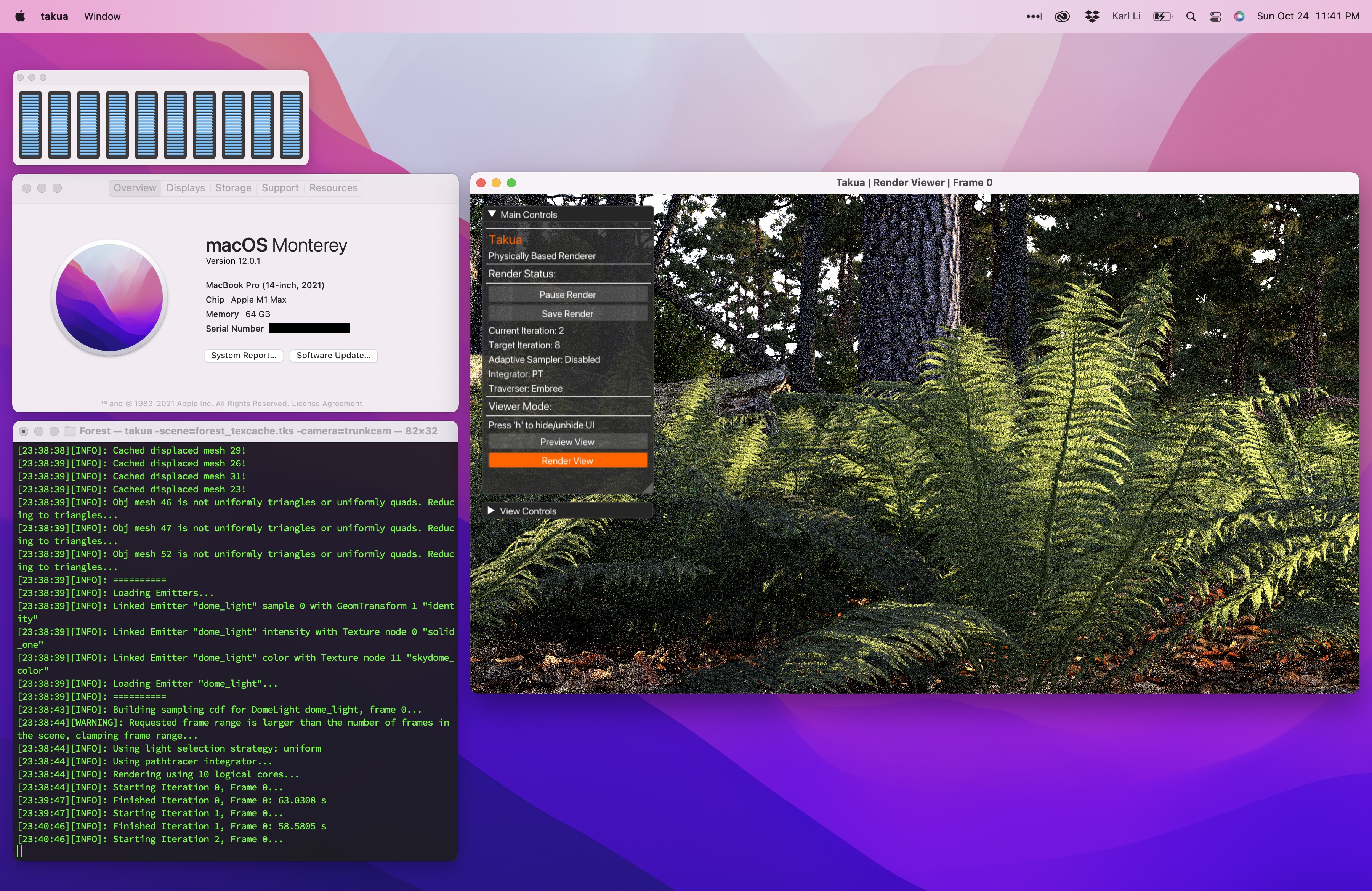


