Mipmapping with Bidirectional Techniques
Table of Contents
Introduction
One major feature that differentiates production-capable renderers from hobby or research renderers is a texture caching system. A well-implemented texture caching system is what allows a production renderer to render scenes with potentially many TBs of textures, but in a reasonable footprint that fits in a few dozen or a hundred-ish GB of RAM. Pretty much every production renderer today has a robust texture caching system; Arnold famously derives a significant amount of performance from an extremely efficient texture cache implementation, and Vray/Corona/Renderman/Hyperion/etc. all have their own, similarly efficient systems.
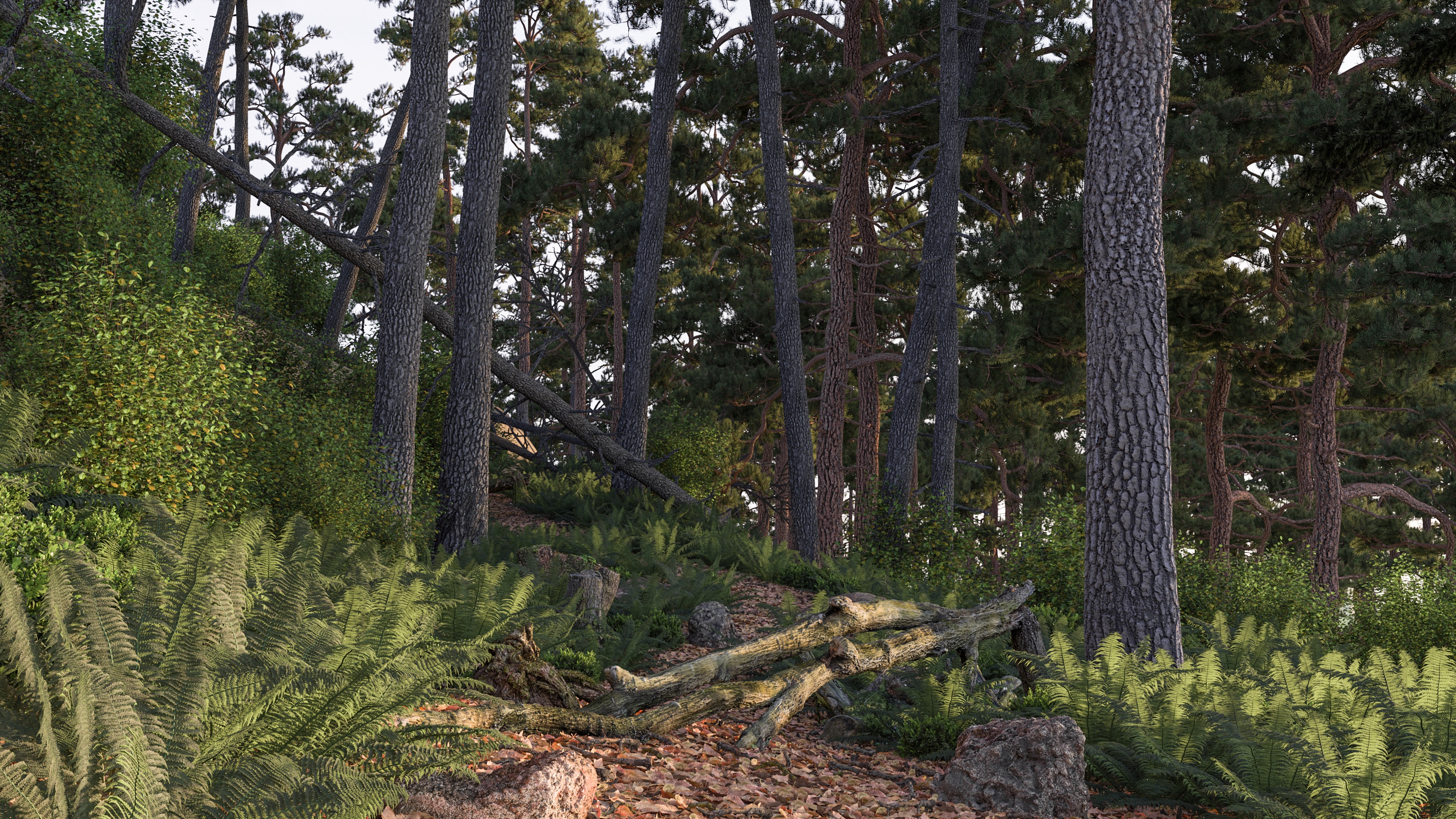
In this post and the next few posts, I’ll write about how I implemented a tiled, mipmapped texture caching system in my hobby renderer, Takua Renderer. I’ll also discuss some of the interesting challenges I ran into along the way. This post will focus on the mipmapping part of the system. Building a tiled mipmapping system that works well with bidirectional path tracing techniques was particularly difficult, for reasons I’ll discuss later in this post. I’ll also review the academic literature on ray differentials and mipmapping with path tracing, and I’ll take a look at what several different production renderers do. The scene I’ll use as an example in this post is a custom recreation of a forest scene from Evermotion’s Archmodels 182, rendered entirely using Takua Renderer (of course):
Texture Caches and Mipmaps
Texture caching is typically coupled with some form of a tiled, mipmapped [Williams 1983] texture system; the texture cache holds specific tiles of an image that were accessed, as opposed to an entire texture. These tiles are typically lazy-loaded on demand into a cache [Peachey 1990], which means the renderer only needs to pay the memory storage cost for only parts of a texture that the renderer actually accesses.
The remainder of this section and the next section of this post are a recap of what mipmaps are, mipmap level selection, and ray differentials for the less experienced reader. I also discuss a bit about what techniques various production renderers are known to use today. If you already know all of this stuff, I’d suggest skipping down a bit to the section titled “Ray Differentials and Bidirectional Techniques”.
Mipmapping works by creating multiple resolutions of a texture, and for a given surface, only loading the last resolution level where the frequency detail falls below the Nyquist limit when viewed from the camera. Since textures are often much more high resolution than the final framebuffer resolution, mipmapping means the renderer can achieve huge memory savings, since for objects further away from the camera, most loaded mip levels will be significantly lower resolution than the original texture. Mipmaps start with the original full resolution texture as “level 0”, and then each level going up from level 0 is half the resolution of the previous level. The highest level is the level at which the texture can no longer be halved in resolution again.
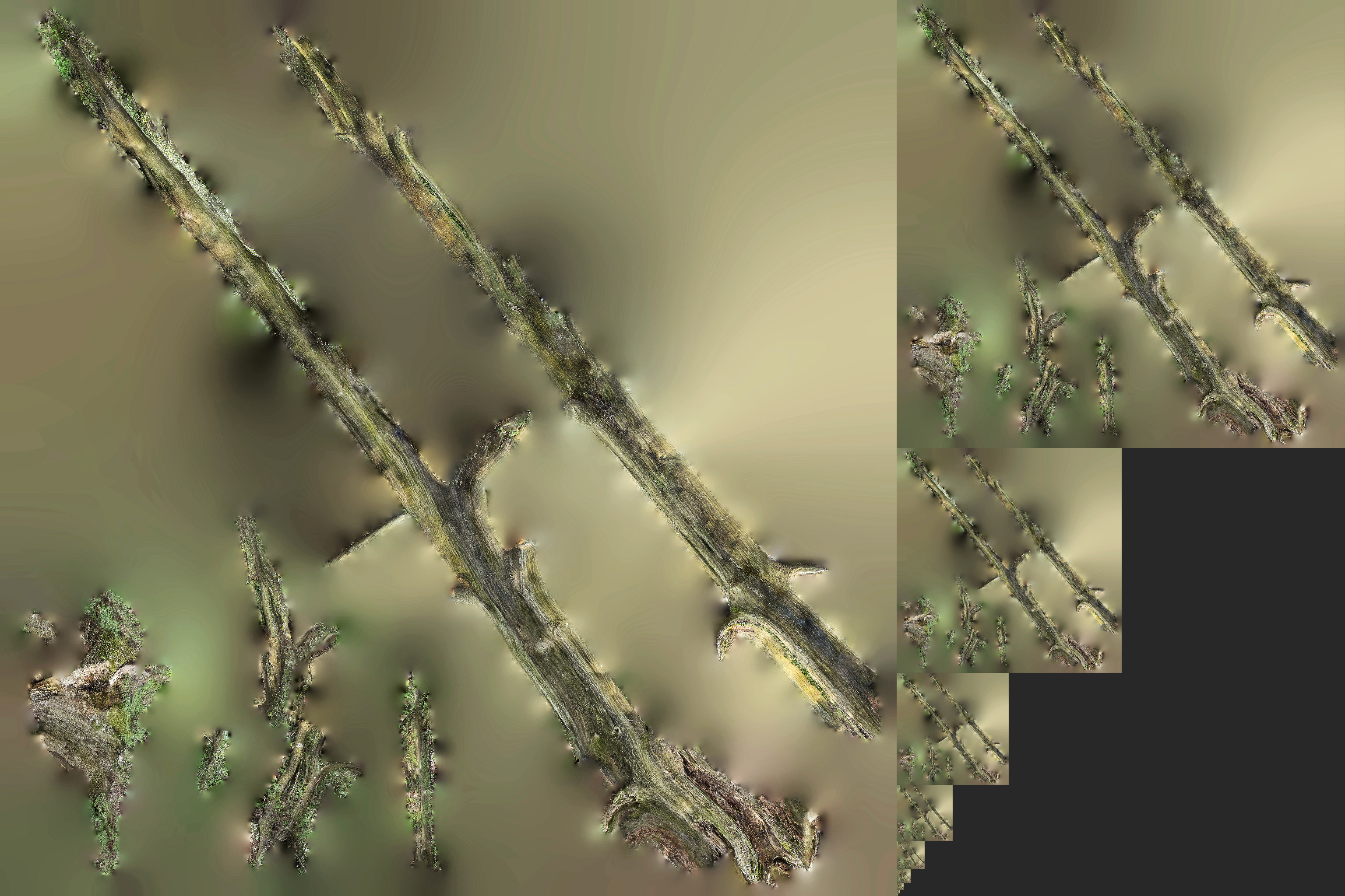
Below is an example of a mipmapped texture. The texture below is the diffuse albedo texture for the fallen log that is in the front of the scene in Figure 1, blocking off the path into the woods. On the left side of Figure 2 is level 1 of this texture (I have omitted level 0 both for image size reasons and because the original texture is from a commercial source, which I don’t have the right to redistribute in full resolution). On the right side, going from the top on down, are levels 2 through 11 of the mipmap. I’ll talk about the “tiled” part in a later post.
Before diving into details, I need to make a major note: I’m not going to write too much about texture filtering for now, mainly because I haven’t done much with texture filtering in Takua at all. Mipmapping was originally invented as an elegant solution to the problem of expensive texture filtering in rasterized rendering; when a texture had detail that was more high frequency than the distance between neighboring pixels in the framebuffer, aliasing would occur when the texture was sampled. Mipmaps are typically generated with pre-computed filtering for mip levels above the original resolution, allowing for single texture samples to appear antialiased. For a comprehensive discussion of texture filtering, how it relates to mipmaps, and more advanced techniques, see section 10.4.3 in Physically Based Rendering 3rd Edition [Pharr et al. 2016].
For now, Takua just uses a point sampler for all texture filtering; my interest in mipmaps is mostly for memory efficiency and texture caching instead of filtering. My thinking is that in a path tracer that is going to generate hundreds or even thousands of paths for each framebuffer pixel, the need for single-sample antialiasing becomes somewhat lessened, since we’re already basically supersampling. Good texture filtering is still ideal of course, but being lazy and just relying on supersampling to get rid of texture aliasing in primary visibility is… not necessarily the worst short-term solution in the world. Furthermore, relying on just point sampling means each texture sample only requires two texture lookups: one from the integer mip level and one from the integer mip level below the continuous float mip level at a sample point (see the next section for more on this). Using only two texture lookups per texture sample is highly efficient due to minimized memory access and minimized branching in the code. Interestingly, the Moonray team at Dreamworks Animation arrived at more or less the same conclusion [Lee et al. 2017]; they point out in their paper that geometric complexity, for all intents and purposes, has an infinite frequency, whereas pre-filtered mipmapped textures are already band limited. As a result, the number of samples required to resolve geometric aliasing should be more than enough to also resolve any texture aliasing. The Moonray team found that this approach works well enough to be their default mode in production.
Mipmap Level Selection and Ray Differentials
The trickiest part of using mipmapped textures is figuring out what mipmap level to sample at any given point. Since the goal is to find a mipmap level with a frequency detail as close to the texture sampling rate as possible, we need to have a sense of what the texture sampling rate at a given point in space relative to the camera will be. More precisely, we want the differential of the surface parameterization (a.k.a. how uv space is changing) with respect to the image plane. Since the image plane is two-dimensional, we will end up with a differential for each uv axis with respect to each axis of the image plane; we call these differentials dudx/dvdx and dudy/dvdy, where u/v are uv coordinates and x/y are image plane pixel coordinates. Calculating these differentials is easy enough in a rasterizer: for each image plane pixel, take the texture coordinate of the fragment and subtract with the texture coordinates of the neighboring fragments to get the gradient of the texture coordinates with respect to the image plane (a.k.a. screen space), and then scale by the texture resolution. Once we have dudx/dvdx and dudy/dvdy, for a non-fancy box filter all we have to do to get the mipmap level is take the longest of these gradients and calculate its logarithm base 2. A code snippet might look something like this:
float mipLevelFromDifferentialSurface(const float dudx,
                                      const float dvdx,
                                      const float dudy,
                                      const float dvdy,
                                      const int maxMipLevel) {
    float width = max(max(dudx, dvdx), max(dudy, dvdy));
    float level = float(maxMipLevel) + log2(width);
    return level;
}
Notice that the level value is a continuous float. Usually, instead of rounding level to an integer, a better approach is to sample both of the integer mipmap levels above and below the continuous level and blend between the two values using the fractional part of level. Doing this blending helps immensely with smoothing transitions between mipmap levels, which can become very important when rendering an animated sequence with camera movement.
In a ray tracer, however, figuring out dudx/dvdx and dudy/dvdy is not as easy as in a rasterizer. If we are only considering primary rays, we can do something similar to the rasterization case: fire a ray from a given pixel and fire rays from the neighboring pixels, and calculate the gradient of the texture coordinates with respect to screen space (the screen space partial derivatives) by examining the hit points of each neighboring ray that hits the same surface as the primary ray. This approach rapidly falls apart though, for the following reasons and more:
- If a ray hits a surface but none of its neighboring rays hit the same surface, then we can’t calculate any differentials and must fall back to point sampling the lowest mip level. This isn’t a problem in the rasterization case, since rasterization will run through all of the polygons that make up a surface, but in the ray tracing case, we only know about surfaces that we actually hit with a ray.
- For secondary rays, we would need to trace secondary bounces not just for a given pixel’s ray, but also its neighboring rays. Doing so would be necessary since, depending on the bsdf at a given surface, the distance between the main ray and its neighbor rays can change arbitrarily. Tracing this many additional rays quickly becomes prohibitively expensive; for example, if we are considering four neighbors per pixel, we are now tracing five times as many rays as before.
- We would also have to continue to guarantee that neighbor secondary rays continue hitting the same surface as the main secondary ray, which will become arbitrarily difficult as bxdf lobes widen or narrow.
A better solution to these problems is to use ray differentials [Igehy 1999], which is more or less just a ray along with the partial derivative of the ray with respect to screen space. Thinking of a ray differential as essentially similar to a ray with a width or a cone, similar to beam tracing [Heckbert and Hanrahan 1984], pencil tracing [Shinya et al. 1987], or cone tracing [Amanatides 1984], is not entirely incorrect, but ray differentials are a bit more nuanced than any of the above. With ray differentials, instead of tracing a bunch of independent neighbor rays with each camera ray, the idea is to reconstruct dudx/dvdy and dudy/dvdy at each hit point using simulated offset rays that are reconstructed using the ray’s partial derivative. Ray differentials are generated alongside camera rays; when a ray is traced from the camera, offset rays are generated for a single neighboring pixel vertically and a single neighboring pixel horizontally in the image plane. Instead of tracing these offset rays independently, however, we always assume they are at some angular width from main ray. When the main ray hits a surface, we need to calculate for later use the differential of the surface at the intersection point with respect to uv space, which is called dpdu and dpdv. Different surface types will require different functions to calculate dpdu and dpdv; for a triangle in a triangle mesh, the code requires the position and uv coordinates at each vertex:
DifferentialSurface calculateDifferentialSurfaceForTriangle(const vec3& p0,
                                                            const vec3& p1,
                                                            const vec3& p2,
                                                            const vec2& uv0,
                                                            const vec2& uv1,
                                                            const vec2& uv2) {
    vec2 duv02 = uv0 - uv2;
    vec2 duv12 = uv1 - uv2;
    float determinant = duv02[0] * duv12[1] - duv02[1] * duv12[0];

    vec3 dpdu, dpdv;

    vec3 dp02 = p0 - p2;
    vec3 dp12 = p1 - p2;
    if (abs(determinant) == 0.0f) {
        vec3 ng = normalize(cross(p2 - p0, p1 - p0));
        if (abs(ng.x) > abs(ng.y)) {
            dpdu = vec3(-ng.z, 0, ng.x) / sqrt(ng.x * ng.x + ng.z * ng.z);
        } else {
            dpdu = vec3(0, ng.z, -ng.y) / sqrt(ng.y * ng.y + ng.z * ng.z);
        }
        dpdv = cross(ng, dpdu);
    } else {
        float invdet = 1.0f / determinant;
        dpdu = (duv12[1] * dp02 - duv02[1] * dp12) * invdet;
        dpdv = (-duv12[0] * dp02 + duv02[0] * dp12) * invdet;
    }
    return DifferentialSurface(dpdu, dpdv);
}
Calculating surface differentials does add a small bit of overhead to the renderer, but the cost can be minimized with some careful work. The naive approach to surface differentials is to calculate them with every intersection point and return them as part of the hit point information that is produced by ray traversal. However, this computation is wasted if the shading operation for a given hit point doesn’t actually end up doing any texture lookups. In Takua, surface differentials are calculated on demand at texture lookup time instead of at ray intersection time; this way, we don’t have to pay the computational cost for the above function unless we actually need to do texture lookups. Takua also supports multiple uv sets per mesh, so the above function is parameterized by uv set ID, and the function is called once for each uv set that a texture specifies. Surface differentials are also cached within a shading operation per hit point, so if a shader does multiple texture lookups within a single invocation, the required surface differentials don’t need to be redundantly calculated.
Sony Imageworks’ variant of Arnold (we’ll refer to it as SPI Arnold to disambiguate from Solid Angle’s Arnold) does something even more advanced [Kulla et al. 2018]. Instead of the above explicit surface differential calculation, SPI Arnold implements an automatic differentiation system utilizing dual arithmetic [Piponi 2004]. SPI Arnold extensively utilizes OSL for shading; this means that they are able to trace at runtime what dependencies a particular shader execution path requires, and therefore when a shader needs any kind of derivative or differential information. The calls to the automatic differentiation system are then JITed into the shader’s execution path, meaning shader authors never have to be aware of how derivatives are computed in the renderer. The SPI Arnold team’s decision to use dual arithmetic based automatic differentiation is influenced by lessons they had previously learned with BMRT’s finite differencing system, which required lots of extraneous shading computations for incoherent ray tracing [Gritz and Hahn 1996]. At least for my purposes, though. I’ve found that the simpler approach I have taken in Takua is sufficiently negligible in both final overhead and code complexity that I’ll probably skip something like the SPI Arnold approach for now.
Once we have the surface differential, we can then approximate the local surface geometry at the intersection point with a tangent plane, and intersect the offset rays with the tangent plane. To find the corresponding uv coordinates for the offset ray tangent plane intersection planes, dpdu/dpdv, the main ray intersection point, and the offset ray intersection points can be used to establish a linear system. Solving this linear system leads us directly to dudx/dudy and dvdx/dvdy; for the exact mathematical details and explanation, see section 10.1 in Physically Based Rendering 3rd Edition. The actual code might look something like this:
// This code is heavily aped from PBRT v3; consult the PBRT book for details!
vec4 calculateScreenSpaceDifferential(const vec3& p,            // Surface intersection point
                                      const vec3& n,            // Surface normal
                                      const vec3& origin,       // Main ray origin
                                      const vec3& rDirection,   // Main ray direction
                                      const vec3& xorigin,      // Offset x ray origin
                                      const vec3& rxDirection,  // Offset x ray direction
                                      const vec3& yorigin,      // Offset y ray origin
                                      const vec3& ryDirection,  // Offset y ray direction
                                      const vec3& dpdu,         // Surface differential w.r.t. u
                                      const vec3& dpdv          // Surface differential w.r.t. v
                                      ) {
    // Compute offset-ray intersection points with tangent plane
    float d = dot(n, p);
    float tx = -(dot(n, xorigin) - d) / dot(n, rxDirection);
    vec3 px = origin + tx * rxDirection;
    float ty = -(dot(n, yorigin) - d) / dot(n, ryDirection);
    vec3 py = origin + ty * ryDirection;
    vec3 dpdx = px - p;
    vec3 dpdy = py - p;

    // Compute uv offsets at offset-ray intersection points
    // Choose two dimensions to use for ray offset computations
    ivec2 dim;
    if (std::abs(n.x) > std::abs(n.y) && std::abs(n.x) > std::abs(n.z)) {
        dim = ivec2(1,2);
    } else if (std::abs(n.y) > std::abs(n.z)) {
        dim = ivec2(0,2);
    } else {
        dim = ivec2(0,1);
    }
    // Initialize A, Bx, and By matrices for offset computation
    mat2 A;
    A[0][0] = ds.dpdu[dim[0]];
    A[0][1] = ds.dpdv[dim[0]];
    A[1][0] = ds.dpdu[dim[1]];
    A[1][1] = ds.dpdv[dim[1]];
    vec2 Bx(px[dim[0]] - p[dim[0]], px[dim[1]] - p[dim[1]]);
    vec2 By(py[dim[0]] - p[dim[0]], py[dim[1]] - p[dim[1]]);

    float dudx, dvdx, dudy, dvdy;

    // Solve two linear systems to get uv offsets
    auto solveLinearSystem2x2 = [](const mat2& A, const vec2& B, float& x0, float& x1) -> bool {
        float det = A[0][0] * A[1][1] - A[0][1] * A[1][0];
        if (abs(det) < (float)constants::EPSILON) {
            return false;
        }
        x0 = (A[1][1] * B[0] - A[0][1] * B[1]) / det;
        x1 = (A[0][0] * B[1] - A[1][0] * B[0]) / det;
        if (std::isnan(x0) || std::isnan(x1)) {
            return false;
        }
        return true;
    };
    if (!solveLinearSystem2x2(A, Bx, dudx, dvdx)) {
        dudx = dvdx = 0.0f;
    }
    if (!solveLinearSystem2x2(A, By, dudy, dvdy)) {
        dudy = dvdy = 0.0f;
    }

    return vec4(dudx, dvdx, dudy, dvdy);
}
Now that we have dudx/dudy and dvdx/dvdy, getting the proper mipmap level works just like in the rasterization case. The above approach is exactly what I have implemented in Takua Renderer for camera rays. Similar to surface differentials, Takua caches dudx/dudy and dvdx/dvdy computations per shader invocation per hit point, so that multiple textures utilizing the same uv set dont’t require multiple redundant calls to the above function.
The ray derivative approach to mipmap level selection is basically the standard approach in modern production rendering today for camera rays. PBRT [Pharr et al. 2016], Mitsuba [Jakob 2010], and Solid Angle’s version of Arnold [Georgiev et al. 2018] all use ray differential systems based on this approach for camera rays. Renderman [Christensen et al. 2018] uses a simplified version of ray differentials that only tracks two floats per ray, instead of the four vectors needed to represent a full ray differential. Renderman tracks a width at each ray’s origin, and a spread value representing the linear rate of change of the ray width over a unit distance. This approach does not encode as much information as the full ray derivative approach, but nonetheless ends up being sufficient since in a path tracer, every pixel essentially ends up being supersampled. Hyperion [Burley et al. 2018] uses a similarly simplified scheme.
A brief side note: being able to calculate the differential for surface normals with respect to screen space is useful for bump mapping, among other things, and the calculation is directly analogous to the pseudocode above for calculateDifferentialSurfaceForTriangle() and calculateScreenSpaceDifferential(), just with surface normals substituted in for surface positions.
Ray Differentials and Path Tracing
We now know how to calculate filter footprints using ray differentials for camera rays, which is great, but what about secondary rays? Without ray differentials for secondary rays, path tracing texture access behavior degrades severely, since secondary rays have to fall back to point sampling textures at the lowest mip level. A number of different schemes exist for calculating filter footprints and mipmap levels for secondary rays; here are a few that have been presented in literature and/or are known to be in use in modern production renderers:
Igehy [1999] demonstrates how to propagate ray differentials through perfectly specular reflection and refraction events, which boil down to some simple extensions to the basic math for optical reflection and refraction. However, we still need a means for handling glossy (so really, non-zero surface roughness), which requires an extended version of ray differentials. Path differentials [Suykens and Willems 2001] consider more than just partial derivatives for each screen space pixel footprint; with path differentials, partial derivatives can also be taken at each scattering event along a number of dimensions. As an example, for handling a arbitrarily shaped BSDF lobe, new partial derivatives can be calculated along some parameter of the lobe that describes the shape of the lobe, which takes the form of a bunch of additional scattering directions around the main ray’s scattering direction. If we imagine looking down the main scattering direction and constructing a convex hull around the additional scattering directions, the result is a polygonal footprint describing the ray differential over the scattering event. This footprint can then be approximated by finding the major and minor axis of the polygonal footprint. While the method is general enough to handle arbitrary factors impacting ray directions, unfortunately it can be fairly complex and expensive to compute in practice, and differentials for some types of events can be very difficult to derive. For this reason, none of the major production renderers today actually use this approach. However, there is a useful observation that can be drawn from path differentials: generally, in most cases, primary rays have narrow widths and secondary rays have wider widths [Christensen et al. 2003]; this observation is the basis of the ad-hoc techniques that most production renderers utilize.
Recently, research has appeared that provides an entirely different, more principled approach to selecting filter footprints, based on covariance tracing [Belcour et al. 2013]. The high-level idea behind covariance tracing is that local light interaction effects such as transport, occlusion, roughness, etc. can all be encoded as 5D covariance matrices, which in turn can be used to determine ideal sampling rates. Covariance tracing builds an actual, implementable rendering algorithm on top of earlier, mostly theoretical work on light transport frequency analysis [Durand et al. 2005]. Belcour et al. [2017] presents an extension to covariance tracing for calculating filter footprints for arbitrary shading effects, including texture map filtering. The covariance-tracing based approach differs from path differentials in two key areas. While both approaches operate in path space, path differentials are much more expensive to compute than the covariance-tracing based technique; path differential complexity scales quadratically with path length, while covariance tracing only ever carries a single covariance matrix along a path for a given effect. Also, path differentials can only be generated starting from the camera, whereas covariance tracing works from the camera and the light; in the next section, we’ll talk about why this difference is critically important.
Covariance tracing based techniques have a lot of promise, and are the best known approach to date for for selecting filter footprints along a path. The original covariance tracing paper had some difficulty with handling high geometric complexity; covariance tracing requires a voxelized version of the scene for storing local occlusion covariance information, and covariance estimates can degrade severely if the occlusion covariance grid is not high resolution enough to capture small geometric details. For huge production scale scenes, geometric complexity requirements can make covariance tracing either slow due to huge occlusion grids, or degraded in quality due to insufficiently large occlusion grids. However, the voxelization step is not as much of a barrier to practicality as it may initially seem. For covariance tracing based filtering, visibility can be neglected, so the entire scene voxelization step can be skipped; Belcour et al. [2017] demonstrates how. Since covariance tracing based filtering can be used with the same assumptions and data as ray differentials but is both superior in quality and more generalizable than ray differentials, I would not be surprised to see more renderers adopt this technique over time.
As of present, however, instead of using any of the above techniques, pretty much all production renderers today use various ad-hoc methods for tracking ray widths for secondary rays. SPI Arnold tracks accumulated roughness values encountered by a ray: if a ray either encounters a diffuse event or reaches a sufficiently high accumulated roughness value, SPI Arnold automatically goes to basically the highest available MIP level [Kulla et al. 2018]. This scheme produces very aggressive texture filtering, but in turn provides excellent texture access patterns. Solid Angle Arnold similarly uses an ad-hoc microfacet-inspired heuristic for secondary rays [Georgiev et al. 2018] . Renderman handles reflection and refraction using something similar to Igehy [1999], but modified for the single-float-width ray differential representation that Renderman uses [Christensen et al. 2018]. For glossy and diffuse events, Renderman uses an empirically determined heuristic where higher ray width spreads are driven by lower scattering direction pdfs. Weta’s Manuka has a unified roughness estimation system built into the shading system, which uses a mean cosine estimate for figuring out ray differentials [Fascione et al. 2018].
Generally, roughness driven heuristics seem to work reasonably well in production, and the actual heuristics don’t actually have to be too complicated! In an experimental branch of PBRT, Matt Pharr found that a simple heuristic that uses a ray differential covering roughly 1/25th of the hemisphere for diffuse events and 1/100th of the hemisphere for glossy events generally worked reasonably well [Pharr 2017].
Ray Differentials and Bidirectional Techniques
So far everything we’ve discussed has been for unidirectional path tracing that starts from the camera. What about ray differentials and mip level selection for paths starting from a light, and by extension, for bidirectional path tracing techniques? Unfortunately, nobody has a good, robust solution for calculating ray differentials for light path! Calculating ray differentials for light paths is fundamentally something of an ill defined problem: a ray differential has to be calculated with respect to a screen space pixel footprint, which works fine for camera paths since the first ray starts from the camera, but for light paths, the last ray in the path is the one that reaches the camera. With light paths, we have something of a chicken-and-egg problem; there is no way to calculate anything with respect to a screen space pixel footprint until a light path has already been fully constructed, but the shading computations required to construct the path are the computations that want differential information in the first place. Furthermore, even if we did have a good way to calculate a starting ray differential from a light, the corresponding path differential can’t become as wide as in the case of a camera path, since at any given moment the light path might scatter towards the camera and therefore needs to maintain a footprint no wider than a single screen space pixel.
Some research work has gone into this question, but more work is needed on this topic. The previously discussed covariance tracing based technique [Belcour et al. 2017] does allow for calculating an ideal texture filtering width and mip level once a light path is fully constructed, but again, the real problem is that footprints need to be available during path construction, not afterwards. With bidirectional path tracing, things get even harder. In order to keep a bidirectional path unbiased, all connections between camera and light path vertices must be consistent in what mip level they sample; however, this is difficult since ray differentials depend on the scattering events at each path vertex. Belcour et al. [2017] demonstrates how important consistent texture filtering between two vertices is.
Currently, only a handful of production renderers have extensive support for bidirectional techniques; of the ones that do, the most common solution to calculating ray differentials for bidirectional paths is… simply not to at all. Unfortunately, this means bidirectional techniques must rely on point sampling the lowest mip level, which defeats the whole point of mipmapping and destroys texture caching performance. The Manuka team alludes to using ray differentials for photon map gather widths in VCM and notes that these ray differentials are implemented as part of their manifold next event estimation system [Fascione et al. 2018], but there isn’t enough detail in their paper to be able to figure out how this actually works.
Camera-Based Mipmap Level Selection
Takua has implementations of standard bidirectional path tracing, progressive photon mapping, and VCM, and I wanted mipmapping to work with all integrator types in Takua. I’m interested in using Takua to render scenes with very high complexity levels using advanced (often bidirectional) light transport algorithms, but reaching production levels of shading complexity without a mipmapped texture cache simply is not possible without crazy amounts of memory (where crazy is defined as in the range of dozens to hundreds of GB of textures or more). However, for the reasons described above, standard ray differential based techniques for calculating mip levels weren’t going to work with Takua’s bidirectional integrators.
The lack of a ray differential solution for light paths left me stuck for some time, until late in 2017, when I got to read an early draft of what eventually became the Manuka paper [Fascione et al. 2018] in the ACM Transactions on Graphics special issue on production rendering. I highly recommend reading all five of the production renderer system papers in the ACM TOG special issue. However, if you’re already generally familiar with how a modern PBRT-style renderer works and only have time to read one paper, I would recommend the Manuka paper simply because Manuka’s architecture and the set of trade-offs and choices made by the Manuka team are so different from what every other modern PBRT-style production path tracer does. What I eventually implemented in Takua is directly inspired by Manuka, although it’s not what Manuka actually does (I think).
The key architectural feature that differentiates Manuka from Arnold/Renderman/Vray/Corona/Hyperion/etc. is its shade-before-hit architecture. I should note here that in this context, shade refers to the pattern generation part of shading, as opposed to the bsdf evaluation/sampling part of shading. The brief explanation (you really should go read the full paper) is that Manuka completely decouples pattern generation from path construction and path sampling, as opposed to what all other modern path tracers do. Most modern path tracers use shade-on-hit, which means pattern generation is lazily evaluated to produce bsdf parameters upon demand, such as when a ray hits a surface. In a shade on hit architecture, pattern generation and path sampling are interleaved, since path sampling depends on the results of pattern generation. Separating out geometry processing from path construction is fairly standard in most modern production path tracers, meaning subdivision/tessellation/displacement happens before any rays are traced, and displacement usually involves some amount of pattern generation. However, no other production path tracer separates out all of pattern generation from path sampling the way Manuka does. At render startup, Manuka runs geometry processing, which dices all input geometry into micropolygon grids, and then runs pattern generation on all of the micropolygons. The result of pattern generation is a set of bsdf parameters that are baked into the micropolygon vertices. Manuka then builds a BVH and proceeds with normal path tracing, but at each path vertex, instead of having to evaluate shading graphs and do texture lookups to calculate bsdf parameters, the bsdf parameters are looked up directly from the pre-calculated cached values baked into the micropolygon vertices. Put another way, Manuka is a path tracer with a REYES-style shader execution model [Cook et al. 1987] instead of a PBRT-style shader execution model; Manuka preserves the grid-based shading coherence from REYES while also giving more flexibility to path sampling and light transport, which no longer have to worry about pattern generation making shading slow.
So how does any of this relate to the bidirectional path tracing mip level selection problem? The answer is: in a shade-before-hit architecture, by the time the renderer is tracing light paths, there is no need for mip level selection because there are no texture lookups required anymore during path sampling. During path sampling, Manuka evaluates bsdfs at each hit point using pre-shaded parameters that are bilinearly interpolated from the nearest micropolygon vertices; all of the texture lookups were already done in the pre-shade phase of the renderer! In other words, at least in principle, a Manuka-style renderer can entirely sidestep the bidirectional path tracing mip level selection problem (although I don’t know if Manuka actually does this or not). Also, in a shade-before-hit architecture, there are no concerns with biasing bidirectional path tracing from different camera/light path vertex connections seeing different mip levels. Since all mip level selection and texture filtering decisions take place before path sampling, the view of the world presented to path sampling is always consistent.
Takua is not a shade-before-hit renderer though, and for a variety of reasons, I don’t plan on making it one. Shade-before-hit presents a number of tradeoffs which are worthwhile in Manuka’s case because of the problems and requirements the Manuka team aimed to solve and meet, but Takua is a hobby renderer aimed at something very different from Manuka. The largest drawback of shade-before-hit is the startup time associated with having to pre-shade the entire scene; this startup time can be quite large, but in exchange, the total render time can be faster as path sampling becomes more efficient. However, in a number of workflows, the time to a full render is not nearly as important as the time to a minimum sample count at which point an artistic decision can be made on a noisy image; beyond this point, full render time is less important as long as it is within a reasonable ballpark. Takua currently has a fast startup time and reaches a first set of samples quickly, and I wanted to keep this behavior. As a result, the question then became: in a shade-on-hit architecture, is there a way to emulate shade-before-hit’s consistent view of the world, where texture filtering decisions are separated from path sampling?
The approach I arrived at is to drive mip level selection based on only a world-space distance-to-camera metric, with no dependency at all on the incoming ray at a given hit point. This approach is… not even remotely novel; in a way, this approach is probably the most obvious solution of all, but it took me a long time and a circuitous path to arrive at for some reason. Here’s the high-level overview of how I implemented a camera-based mip level selection technique:
- At render startup time, calculate a ray differential for each pixel in the camera’s image plane. The goal is to find the narrowest differential in each screen space dimension x and y. Store this piece of information for later.
- At each ray-surface intersection point, calculate the differential surface.
- Create a ‘fake’ ray going from the camera’s origin position to the current intersection point, with a ray differential equal to the minimum differential in each direction found in step 1.
- Calculate dudx/dudy and dvdx/dvdy using the usual method presented above, but using the fake ray from step 3 instead of the actual ray.
- Calculate the mip level as usual from dudx/dudy and dvdx/dvdy.
The rational for using the narrowest differentials in step 1 is to guarantee that texture frequency remains sub-pixel for the all pixels in screen space, even if that means that we might be sampling some pixels at a higher resolution mip level than whatever screen space pixel we’re accumulating radiance too. In this case, being overly conservative with our mip level selection is preferable to visible texture blurring from picking a mip level that is too low resolution.
Takua uses the above approach for all path types, including light paths in the various bidirectional integrators. Since the mip level selection is based entirely on distance-to-camera, as far as the light transport integrators are concerned, their view of the world is entirely consistent. As a result, Takua is able to sidestep the light path ray differential problem in much the same way that a shade-before-hit architecture is able to. There are some particular implementation details that are slightly complicated by Takua having support for multiple uv sets per mesh, but I’ll write about multiple uv sets in a later post. Also, there is one notable failure scenario, which I’ll discuss more in the results section.
Results
So how well does camera-based mipmap level selection work compared to a more standard approach based on path differentials or ray widths from the incident ray? Typically in a production renderer, mipmaps work in conjunction with tiled textures, where tiles are a fixed size (unless a tile is in a mipmap level with a total resolution smaller than the tile resolution). Therefore, the useful metric to compare is how many texture tiles each approach access throughout the course of a render; the more an approach accesses higher mipmap levels (meaning lower resolution mipmap levels), the fewer tiles in total should be accessed since lower resolution mipmap levels have fewer tiles.
For unidirectional path tracing from the camera, we can reasonably expect the camera-based approach to perform less well than a path differential or ray width technique (which I’ll call simply ‘ray-based’). In the camera-based approach, every texture lookup has to use a footprint corresponding to approximately a single screen space pixel footprint, whereas in a more standard ray-based approach, footprints get wider with each successive bounce, leading to access to higher mipmap levels. Depending on how aggressively ray widths are widened at diffuse and glossy events, ray-based approaches can quickly reach the highest mipmap levels and essentially spend the majority of the render only accessing high mipmap levels.
For bidirectional integrators though, the camera-based techinque has the major advantage of being able to provide reasonable mipmap levels for both camera and light paths, whereas the more standard ray-based approaches have to fall back to point sampling the lowest mipmap level for light paths. As a result, for bidirectional paths we can expect that a ray-based approach should perform somewhere in between how a ray-based approach performs in the unidirectional case and how point sampling only the lowest mipmap level performs in the unidirectional case.
As a baseline, I also implemented a ray-based approach with a relatively aggressive widening heuristic for glossy and diffuse events. For the forest scene from Figure 1, I got the following results at 1920x1080 resolution with 16 samples per pixel. I compared unidirectional path tracing from the camera and standard bidirectional path tracing; statistics are presented as total number of texture tiles accessed divided by total number of texture tiles across all mipmap levels. The lower the percentage, the better:
16 SPP 1920x1080 Unidirectional (PT)
    No mipmapping:                       314439/745394 tiles (42.18%)
    Ray-based level selection:           103206/745394 tiles (13.84%)
    Camera-based level selection:        104764/745394 tiles (14.05%)

16 SPP 1920x1080 Bidirectional (BDPT)
    No mipmapping:                       315452/745394 tiles (42.32%)
    Ray-based level selection:           203491/745394 tiles (27.30%)
    Camera-based level selection:        104858/745394 tiles (14.07%)
As expected, in the unidirectional case, the camera-based approach accesses slightly more tiles than the ray-based approach, and both approaches significantly outperform point sampling the lowest mipmap level. In the bidirectional case, the camera-based approach accesses slightly more tiles than in the unidirectional case, while the ray-based approach performs somewhere between the ray-based approach in unidirectional and point sampling the lowest mipmap level in unidirectional. What surprised me is how close the camera-based approach performed compared to the ray-based approach in the unidirectional case, especially since I chose a fairly aggresive widening heuristic (essentially a more aggressive version of the same heuristic that Matt Pharr uses in the texture cached branch of PBRTv3).
To help with visualizing what mipmap levels are being accessed, I implemented a new AOV in Takua that assigns colors to surfaces based on what mipmap level is accessed. With camera-based mipmap level selection, this AOV shows simply what mipmap level is accessed by all rays that hit a given point on a surface. Each mipmap level is represented by a different color, with support up to 12 mipmap levels. The following two images show accessed mipmap level at 1080p and 2160p (4K); note how the 2160p render accesses more lower mipmap levels than the 1080p render. The pixel footprints in the higher resolution render are smaller when projected into world space since more pixels have to pack into the same field of view. The key below each image shows what mipmap level each color corresponds to:
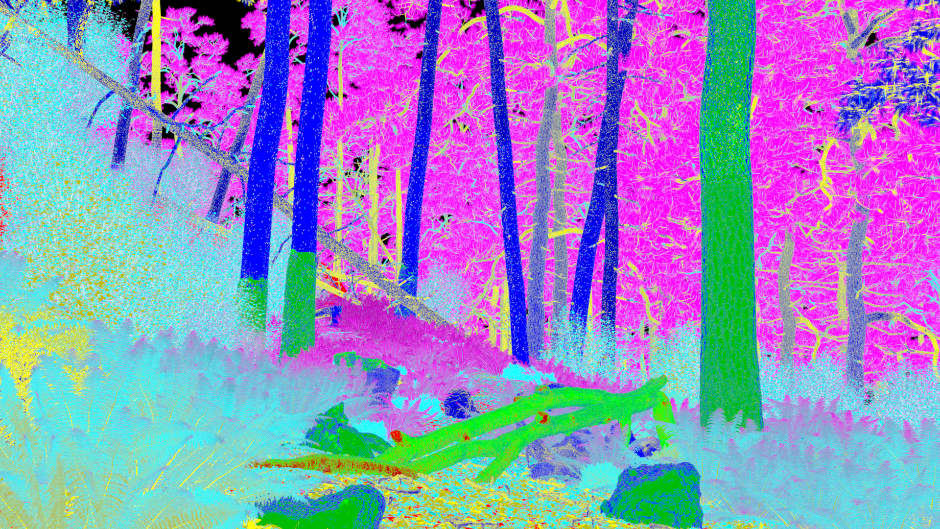
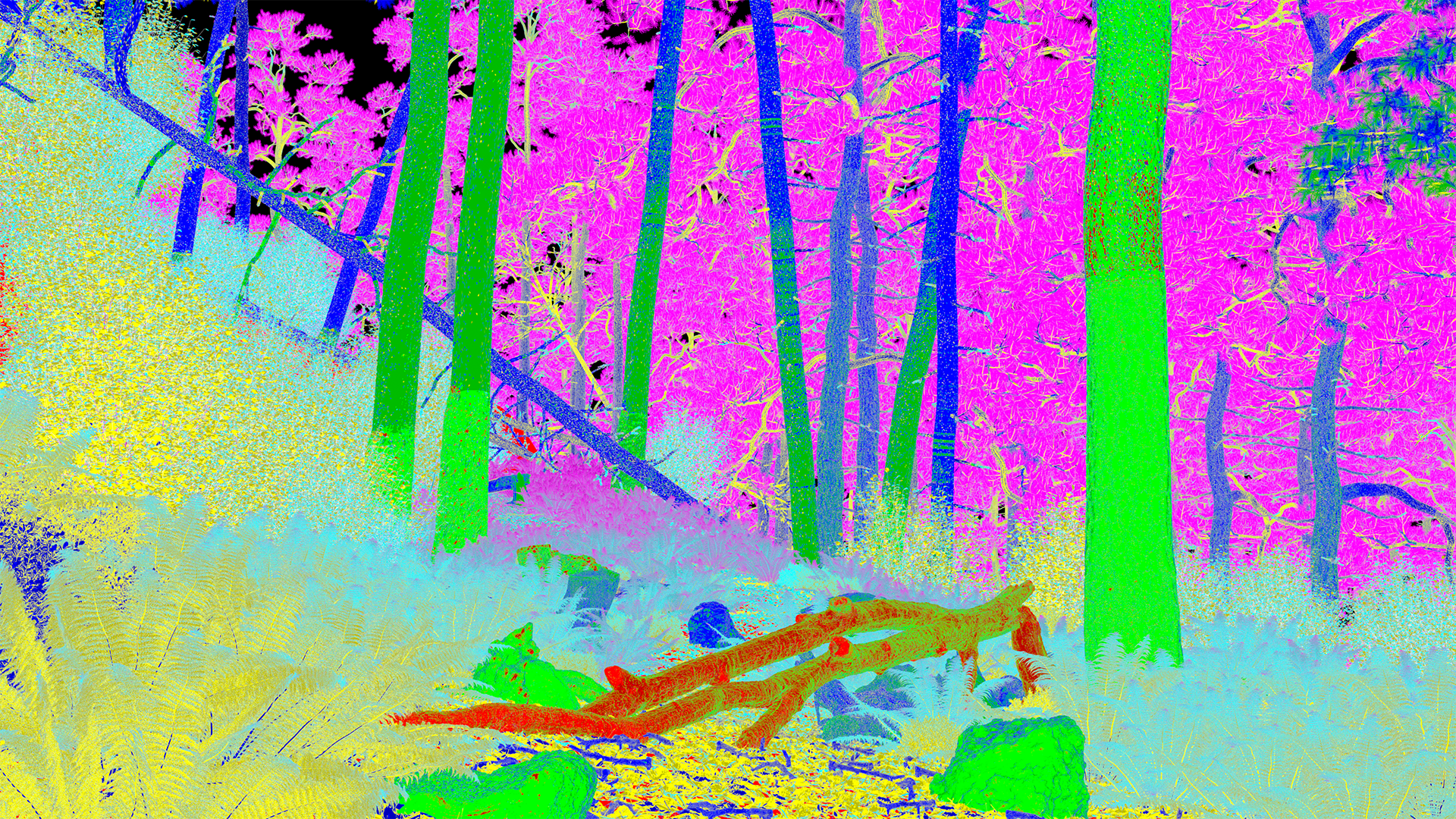
In general, everything looks as we would expect it to look in a working mipmapping system! Surface points farther away from the camera are generally accessing higher mipmap levels, and surface points closer to the camera are generally accessing lower mipmap levels. The ferns in the front of the frame near the camera access higher mipmap levels than the big fallen log in the center of the frame even though the ferns are closer to the camera because the textures for each leaf are extremely high resolution and the fern leaves are very small in screen-space. Surfaces that are viewed at highly glancing angles from the camera tend to access higher mipmap levels than surfaces that are camera-facing; this effect is easiest to see on the rocks in bottom front of the frame. The interesting sudden shift in mipmap level on some of the tree trunks comes from the tree trunks using two diffrent uv sets; the lower part of each tree trunk uses a different texture than the upper part, and the main textures are blended using a blending mask in a different uv space from the main textures; since the differential surface depends in part on the uv parameterization, different uv sets can result in different mipmap level selection behavior.
I also added a debug mode to Takua that tracks mipmap level access per texture sample. In this mode, for a given texture, the renderer splats into an image the lowest acceessed mipmap level for each texture sample. The result is sort of a heatmap that can be overlaid on the original texture’s lowest mipmap level to see what parts of texture are sampled at what resolution. Figure 5 shows one of these heatmaps for the texture on the fallen log in the center of the frame:
Just like in Figures 3 and 4, we can see that renders at higher resolutions will tend to access lower mipmap levels more frequently. Also, we can see that the vast majority of the texture is never sampled at all; with a tiled texture caching system where tiles are loaded on demand, this means there are a large number of texture tiles that we never bother to load at all. In cases like Figure 5, not loading unused tiles provides enormous memory savings compared to if we just loaded an entire non-mipmapped texture.
So far using a camera-based approach to mipmap level selection combined with just point sampling at each texture sample has held up very well in Takua! In fact, the Scandinavian Room scene from earlier this year was rendered using the mipmap approach described in this post as well. There is, however, a relatively simple type of scene that Takua’s camera-based approach fails badly at handling: refraction near the camera. If a lens is placed directly in front of the camera that significantly magnifies part of the scene, a purely world-space metric for filter footprints can result in choosing mipmap levels that are too high, which translates to visible texture blurring or pixelation. I don’t have anything implemented to handle this failure case right now. One possible solution I’ve thought about is to initially trace a set of rays from the camera using traditional ray differential propogation for specular objects, and cache the resultant mipmap levels in the scene. Then, during the actual renders, the renderer could compare the camera-based metric from the nearest N cached metrics to infer if a lower mipmap level is needed than what the camera-based metric produces. However, such a system would add significant cost to the mipmap level selection logic, and there are a number of implementation complications to consider. I do wonder how Manuka handles the “lens in front of a camera” case as well, since the shade-before-hit paradigm also fails on this scenario for the same reasons.
Long term, I would like to spend more time looking in to (and perhaps implementing) a covariance tracing based approach. While Takua currently gets by with just point sampling, filtering becomes much more important for other effects, such as glinty microfacet materials, and covariance tracing based filtering seems to be the best currently known solution for these cases.
In an upcoming post, I’m aiming to write about how Takua’s texture caching system works in conjunction with the mipmapping system described in this post. As mentioned earlier, I’m also planning a (hopefully) short-ish post about supporting multiple uv sets, and how that impacts a mipmapping and texture caching system.
Additional Renders
Finally, since this has been a very text-heavy post, here are some bonus renders of the same forest scene under different lighting conditions. When I was setting up this scene for Takua, I tried a number of different lighting conditions and settled on the one in Figure 1 for the main render, but some of the alternatives were interesting too. In a future post, I’ll show a bunch of interesting renders of this scene from different camera angles, but for now, here is the forest at different times of day:


References
John Amanatides. 1984. Ray Tracing with Cones. ACM SIGGRAPH Computer Graphics (Proc. of SIGGRAPH) 18, 3 (Jul. 1984), 129-135.
Laurent Belcour, Cyril Soler, Kartic Subr, Nicolas Holzschuch, and Frédo Durand. 2013. 5D Covariance Tracing for Efficient Defocus and Motion Blur. ACM Transactions on Graphics 32, 3 (Jun. 2013), Article 31.
Laurent Belcour, Ling-Qi Yan, Ravi Ramamoorthi, and Derek Nowrouzezahrai. 2017. Antialiasing Complex Global Illumination Effects in Path-Space. ACM Transactions on Graphics 36, 1 (Jan. 2017), Article 9.
Brent Burley, David Adler, Matt Jen-Yuan Chiang, Hank Driskill, Ralf Habel, Patrick Kelly, Peter Kutz, Yining Karl Li, and Daniel Teece. 2018. The Design and Evolution of Disney’s Hyperion Renderer. ACM Transactions on Graphics 37, 3 (Jul. 2018), Article 33.
Per Christensen, Julian Fong, Jonathan Shade, Wayne Wooten, Brenden Schubert, Andrew Kensler, Stephen Friedman, Charlie Kilpatrick, Cliff Ramshaw, Marc Bannister, Brenton Rayner, Jonathan Brouillat, and Max Liani. 2018. RenderMan: An Advanced Path-Tracing Architeture for Movie Rendering. ACM Transactions on Graphics 37, 3 (Jul. 2018), Article 30.
Per Christensen, David M. Laur, Julian Fong, Wayne Wooten, and Dana Batali. 2003. Ray Differentials and Multiresolution Geometry Caching for Distribution Ray Tracing in Complex Scenes. Computer Graphics Forum (Proc. of Eurographics) 22, 3 (Sep. 2003), 543-552.
Robert L. Cook, Loren Carpenter, and Edwin Catmull. 1987. The Reyes Image Rendering Architecture. ACM SIGGRAPH Computer Graphics (Proc. of SIGGRAPH) 21, 4 (Jul. 1987), 95-102.
Frédo Durand, Nicolas Holzchuch, Cyril Soler, Eric Chan, and François X Sillion. 2005. A Frequency Analysis of Light Transport. ACM Transactions on Graphics (Proc. of SIGGRAPH) 24, 3 (Aug. 2005), 1115-1126.
Luca Fascione, Johannes Hanika, Mark Leone, Marc Droske, Jorge Schwarzhaupt, Tomáš Davidovič, Andrea Weidlich and Johannes Meng. 2018. Manuka: A Batch-Shading Architecture for Spectral Path Tracing in Movie Production. ACM Transactions on Graphics 37, 3 (Jul. 2018), Article 31.
Iliyan Georgiev, Thiago Ize, Mike Farnsworth, Ramón Montoya-Vozmediano, Alan King, Brecht van Lommel, Angel Jimenez, Oscar Anson, Shinji Ogaki, Eric Johnston, Adrien Herubel, Declan Russell, Frédéric Servant, and Marcos Fajardo. 2018. Arnold: A Brute-Force Production Path Tracer. ACM Transactions on Graphics 37, 3 (Jul. 2018), Article 32.
Larry Gritz and James K. Hahn. 1996. BMRT: A Global Illumination Implementation of the RenderMan Standard. Journal of Graphics Tools 1, 3 (Jul. 1996), 29-47.
Paul S. Heckbert and Pat Hanrahan. 1984. Beam Tracing Polygonal Objects. ACM SIGGRAPH Computer Graphics (Proc. of SIGGRAPH) 18, 3 (Jul. 1984), 119-127.
Homan Igehy. 1999. Tracing Ray Differentials. In Proc. of SIGGRAPH (SIGGRAPH 1999). 179–186.
Wenzel Jakob. 2010. Mitsuba Renderer.
Christopher Kulla, Alejandro Conty, Clifford Stein, and Larry Gritz. 2018. Sony Pictures Imageworks Arnold. ACM Transactions on Graphics 37, 3 (Jul. 2018), Article 29.
Mark Lee, Brian Green, Feng Xie, and Eric Tabellion. 2017. Vectorized Production Path Tracing. In Proc. of High Performance Graphics (HPG 2017). Article 10.
Darwyn Peachey. 1990. Texture on Demand. Pixar Technical Report 217.
Matt Pharr, Wenzel Jakob, and Greg Humphreys. 2016. Physically Based Rendering: From Theory to Implementation, 3rd ed. Morgan Kaufmann.
Matt Pharr. 2017. The Implementation of a Scalable Texture Cache. Physically Based Rendering Supplemental Material.
Dan Piponi. 2004. Automatic Differentiation, C++ Templates and Photogrammetry. Journal of Graphics Tools 9, 4 (Sep. 2004), 41-55.
Mikio Shinya, Tokiichiro Takahashi, and Seiichiro Naito. 1987. Principles and Applications of Pencil Tracing. ACM SIGGRAPH Computer Graphics (Proc. of SIGGRAPH) 21, 4 (Jul. 1987), 45-54.
Frank Suykens and Yves. D. Willems. 2001. Path Differentials and Applications. In Proc. of Eurographics Workshop on Rendering (Rendering Techniques 2001). 257–268.
Lance Williams. 1983. Pyramidal Parametrics. ACM SIGGRAPH Computer Graphics (Proc. of SIGGRAPH) 12, 3 (Jul. 1983), 1-11.