Adaptive sampling is a relatively small and simple but very powerful feature, so I thought I’d write briefly about how adaptive sampling works in Takua a0.5. Before diving into the details though, I’ll start with a picture. The scene I’ll be using for comparisons in this post is a globe of the Earth, made of a polished ground glass with reflective metal insets for the landmasses and with a rough scratched metal stand. The globe is on a white backdrop and is lit by two off-camera area lights. The following render is the fully converged reference baseline for everything else in the post, rendered using VCM:

As mentioned before, in pathtracing based renderers, we solve the path integral through Monte Carlo sampling, which gives us an estimate of the total integral per sample thrown. As we throw more and more samples at the scene, we get a better and better estimate of the total integral, which explains why pathtracing based integrators start out producing a noisy image but eventually converge to a nice, smooth image if enough rays are traced per pixel.

In a naive renderer, the number of samples traced per pixel is usually just a fixed number, equal for all pixels. However, not all parts of the image are necessarily equally difficult to sample; for example, in the globe scene, the backdrop should require fewer samples than the ground glass globe to converge, and the ground glass globe in turn should require fewer samples than the two caustics on the ground. This observation means that a fixed sampling strategy can potentially be quite wasteful. Instead, computation can be used much more efficiently if the sampling strategy can adapt and drive more samples towards pixels that require more work to converge, while driving fewer samples towards pixels that have already converged mid-render. Such a sample can also be used to automatically stop the renderer once the sampler has detected that the entire render has converged, without needing user guesswork for how many samples to use.

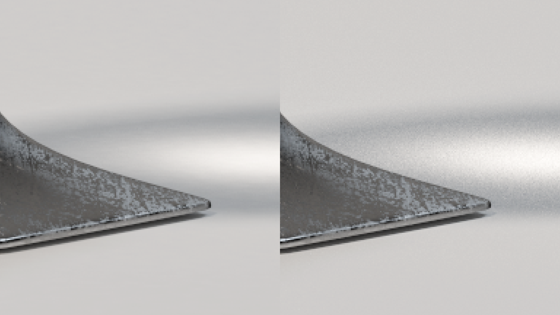
The following image is the same globe scene as above, but limited to 5120 samples per pixel using bidirectional pathtracing and a fixed sampler. Note that most of the image is reasonable converged, but there is still noise visible in the caustics:

Since it may be difficult to see the difference between this image and the baseline image on smaller screens, here is a close-up crop of the same caustic area between the two images:

The difficult part of implementing an adaptive sampler is, of course, figuring out a metric for convergence. The PBRT book presents a very simple adaptive sampling strategy on page 388 of the 2nd edition: for each pixel, generate some minimum number of initial samples and record the radiances returned by each initial sample. Then, take the average of the luminances of the returned radiances, and compute the contrast between each initial sample’s radiance and the average luminance. If any initial sample has a contrast from the average luminance above some threshold (say, 0.5), generate more samples for the pixel up until some maximum number of samples per pixel is reached. If all of the initial samples have contrasts below the threshold, then the sampler can mark the pixel as finished and move onto the next pixel. The idea behind this strategy is to try to eliminate fireflies, since fireflies result from statistically improbably samples that are significantly above the true value of the pixel.

The PBRT adaptive sampler works decently, but has a number of shortcomings. First, the need to draw a large number of samples per pixel simultaneously makes this approach less than ideal for progressive rendering; while well suited to a bucketed renderer, a progressive renderer prefers to draw a small number of samples per pixel per iteration, and return to each pixel to draw more samples in subsequent iterations. In theory, the PBRT adaptive sampler could be made to work with a progressive renderer if sample information was stored from each iteration until enough samples were accumulated to run an adaptive sampling check, but this approach would require storing a lot of extra information. Second, while the PBRT approach can guarantee some degree of per-pixel variance minimization, each pixel isn’t actually aware of what its neighbours look like, meaning that there still can be visual noise across the image. A better, global approach would have to take into account neighbouring pixel radiance values as a second check for whether or not a pixel is sufficiently sampled.

My first attempt at a global approach (the test scene in this post is a globe, but that pun was not intended) was to simply have the adaptive sampler check the contrast of each pixel with it’s immediate neighbours. Every N samples, the adaptive sampler would pull the accumulated radiances buffer and flag each pixel as unconverged if the pixel has a contrast greater than some threshold from at least one of its neighbours. Pixels marked unconverged are sampled for N more iterations, while pixels marked as converged are skipped for the next N iterations. After another N iterations, the adaptive sampler would go back and reflag every pixel, meaning that a pixel previously marked as converged could be reflagged as unconverged if its neighbours changed enormously. Generally N should be a rather large number (say, 128 samples per pixel), since doing convergence checks is meaningless if the image is too noisy at the time of the check.

Using this strategy, I got the following image, which was set to run for a maximum of 5120 samples per pixel but wound up averaging 4500 samples per pixel, or about a 12.1% reduction in samples needed:

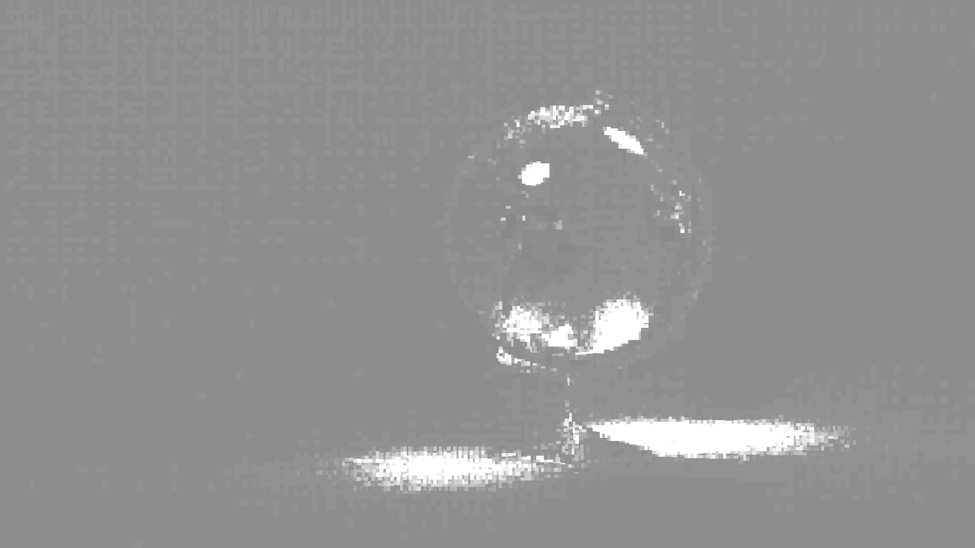
At an initial glance, this looks pretty good! However, as soon as I examined where the actual samples went, I realized that this strategy doesn’t work. The following image is a heatmap showing where samples were driven, with brighter areas indicating more samples per pixel:

Generally, my per-pixel adaptive sampler did correctly identify the caustic areas as needing more samples, but a problem becomes apparent in the backdrop areas: the per-pixel adaptive sampler drove samples at clustered “chunks” evenly, but not evenly across different clusters. This behavior happens because while the per-pixel sampler is now taking into account variance across neighbours, it still doesn’t have any sort of global sense across the entire image! Instead, the sampler is finding localized pockets where variance seems even across pixels, but those pockets can be quite disconnected from further out areas. While the resultant render looks okay at a glance, clustered variance patterns becomes apparent if the image contrast is increased:

Interestingly, these artifacts are reminiscent of the artifacts that show up in not-fully-converged Metropolis Light Transport renders. This similarity makes sense, since in both cases they arise from uneven localized convergence.

The next approach that I tried is a more global approach adapted from Dammertz et al.’s paper, “A Hierarchical Automatic Stopping Condition for Monte Carlo Global Illumination”. For the sake of simplicity, I’ll refer to the approach in this paper as Dammertz for the rest of this post. Dammertz works by considering the variance across an entire block of pixels at once and flagging the entire block as converged or unconverged, allowing for much more global analysis. At the first variance check, the only block considered is the entire image as one enormous block; if the total variance e_b in the entire block is below a termination threshold e_t, the block is flagged as converged and no longer needs to be sampled further. If e_b is greater than e_t but still less than a splitting threshold e_s, then the block will be split into two non-overlapping child blocks for the next round of variance checking after N iterations have passed. At each variance check, this process is repeated for each block, meaning the image eventually becomes split into an ocean of smaller blocks. Blocks are kept inside of a simple unsorted list, require no relational information to each other, and are removed from the list once marked as converged, making the memory requirements very simple. Blocks are split along their major axis, with the exact split point chosen to keep error as equal as possible across the two sides of the split.

The actual variance metric used is also very straightforward; instead of trying to calculate an estimate of variance based on neighbouring pixels, Dammertz stores two framebuffers: one buffer I for all accumulated radiances so far, and a second buffer A for accumulated radiances from every other iteration. As the image approaches full convergence, the differences between I and A should shrink, so an estimation of variance can be found simply by comparing radiance values between I and A. The specific details and formulations can be found in section 2.1 of the paper.

I made a single modification to the paper’s algorithm: I added a lower bound to the block size. Instead of allowing blocks to split all the way to a single pixel, I stop splitting after a block reaches 64 pixels in a 8x8 square. I found that splitting down to single pixels could sometimes cause false positives in convergence flagging, leading to missed pixels similar to in the PBRT approach. Forcing blocks to stop splitting at 64 pixels means there is a chance of false negatives for convergence, but a small amount of unnecessary oversampling is preferable to undersampling.

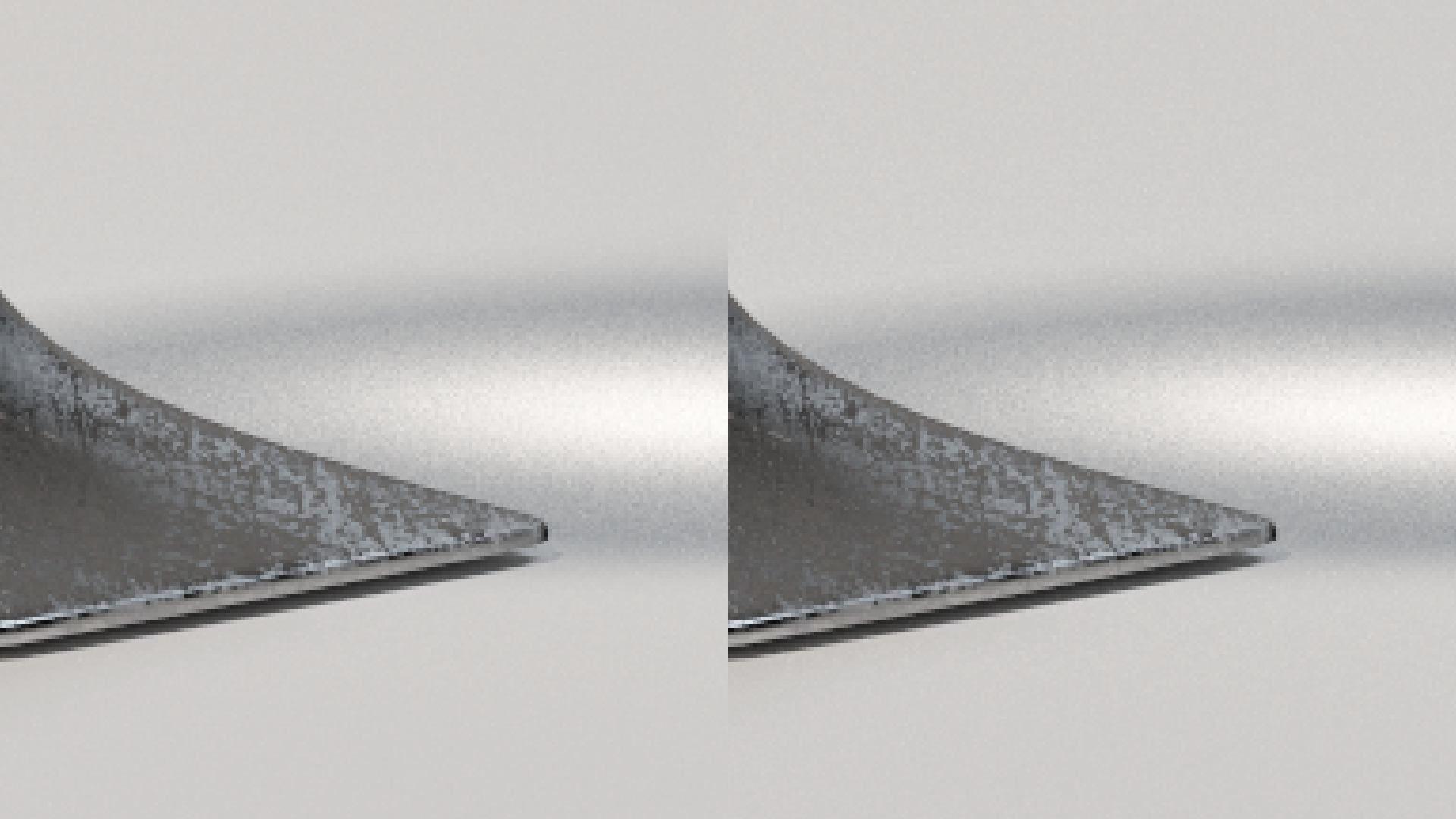
Using this per-block adaptive sampler, I got the following image, which again is superficially extremely similar to the fixed sampler result. This render was also set to run for a maximum of 5120 samples, but wound up averaging just 2920 samples per pixel, or about a 42.9% reduction in samples needed:

The sample heatmap looks good too! The heatmap shows that the sampler correctly identified the caustic and highlight areas as needing more samples, and doesn’t have clustering issues in areas that needed fewer samples:

Boosting the image contrast shows that the image is free of local clustering artifacts and noise is even across the entire image, which is what we would expect:

Looking at the same 500% crop area as earlier, the adaptive per-block and fixed sampling renders are indistinguishable:

So with that, I think Dammertz works pretty well! Also, the computational and memory overhead required for the Dammertz approach is basically negligible relative to the actual rendering process. This approach is the one that is currently in Takua a0.5.

I actually have an additional adaptive sampling trick designed specifically for targeting fireflies. This additional trick works in conjunction with the Dammertz approach. However, this post is already much longer than I originally planned, so I’ll save that discussion for a later post. I’ll also be getting back to the PPM/VCM posts in my series of integrator posts shortly; I have not had much time to write on my blog since the vast majority of my time is currently focused on my thesis, but I’ll try to get something posted soon!