Working Towards Importance Sampled Direct Lighting
I haven’t made a post in a few weeks now since I’ve been working on a number of different things all of which aren’t quite done yet. Since its been a few weeks, here’s a writeup of one of the things I’m working on and where I am with that.
One of the major features I’ve been working towards for the past few weeks is full multiple importance sampling, which will serve a couple of purposes. First, importance sampling the direct lighting contribution in the image should allow for significantly higher convergence rates for the same amount of compute, allowing for much smoother renders for the same render time. Second, MIS will serve as groundwork for future bidirectional integration schemes, such as Metropolis transport and photon mapping. I’ve been working with my friend Xing Du on understanding the math behind MIS and figuring out how exactly the math should translate into implementation.
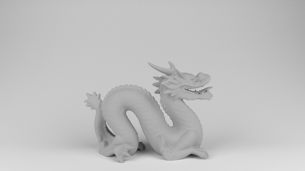
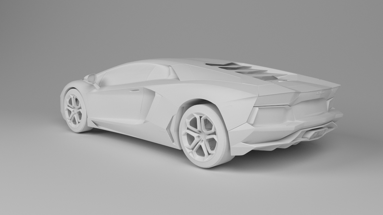
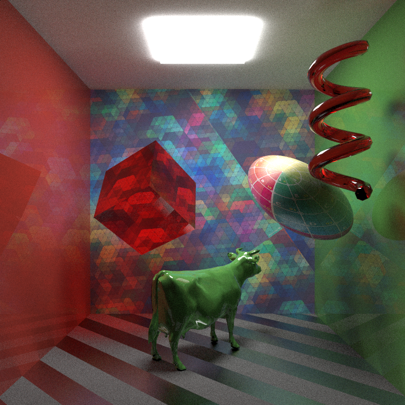
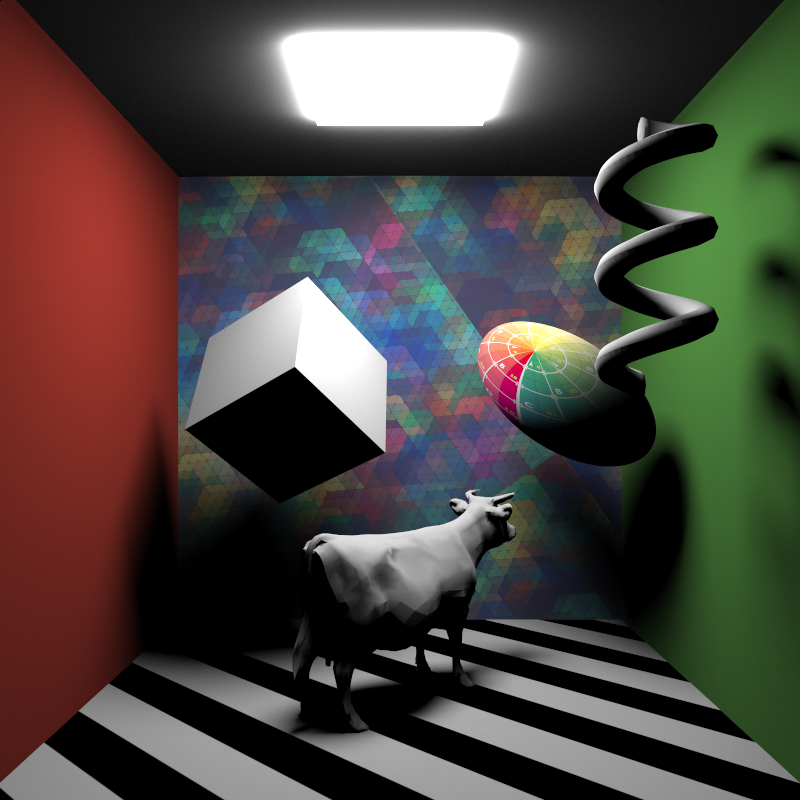
So first off, some ground truth tests. All ground truth tests are rendered using brute force pathtracing with hundreds of thousands of iterations per pixel. Here is the test scene I’ve been using lately, with all surfaces reduced to lambert diffuse for the sake of simplification:
The motivation behind importance sampling lights by directly sampling objects with emissive materials comes from the difficulty of finding useful samples from the BRDF only; for example, for the lambert diffuse case, since sampling from only the BRDF produces outgoing rays in totally random (or, slightly better, cosine weighted random) directions, the probability of any ray coming from a diffuse surface actually hitting a light is relatively low, meaning that the contribution of each sample is likely to be low as well. As a result, finding the direct lighting contribution via just BRDF sampling.
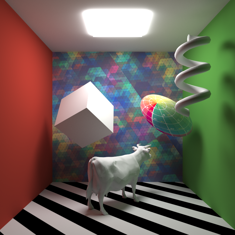
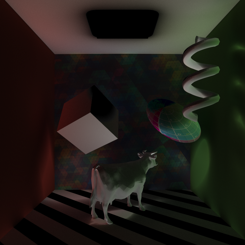
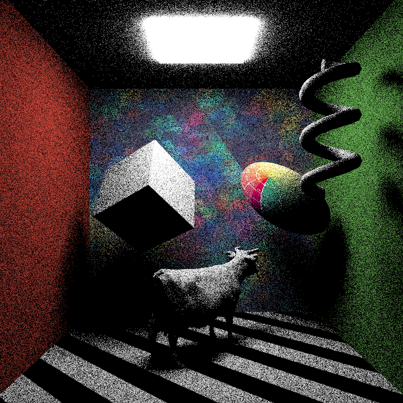
For example, here’s the direct lighting contribution only, after 64 samples per pixel with only BRDF sampling:
Instead of sampling direct lighting contribution by shooting a ray off in a random direction and hoping that maybe it will hit a light, a much better strategy would be to… shoot the ray towards the light source. This way, the contribution from the sample is guaranteed to be useful. There’s one hitch though: the weighting for a sample chosen using the BRDF is relatively simple to determine. For example, in the lambert diffuse case, since the probability of any particular random sample within a hemisphere is the same as any other sample, the weighting per sample is even with all other samples. Once we selectively choose the ray direction specifically towards the light though, the weighting per sample is no longer even. Instead, we must weight each sample by the probability of a ray going in that particular direction towards the light, which we can calculate by the solid angle subtended by the light source divided by the total solid angle of the hemisphere.
So, a trivial example case would be if a point was being lit by a large area light subtending exactly half of the hemisphere visible from the point. In this case, the area light subtends Pi steradians, making its total weight Pi/(2*Pi), or one half.
The tricky part of calculating the solid angle weighting is in calculating the fractional unit-spherical surface area projection for non-uniform light sources. In other words, figuring out what solid angle a sphere subtends is easy, but figuring out what solid angle a Stanford Bunny subtends is…. less easy.
The initial approach that Xing and I arrived at was to break complex meshes down into triangles and treat each triangle as a separate light, since calculating the solid angle subtended by a triangle is once again easy. However, since treating a mesh as a cloud of triangle area lights is potentially very expensive, for each iteration the direct lighting contribution from all lights in the scene becomes potentially untenable, meaning that each iteration of the render will have to randomly select a small number of lights to directly sample.
As a result, we brainstormed some ideas for potential shortcuts. One shortcut idea we came up with was that instead of choosing an evenly distributed point on the surface of the light to serve as the target for our ray, we could instead shoot a ray at the bounding sphere for the target light and weight the resulting sample by the solid angle subtended not by the light itself, but by the bounding sphere. Our thinking was that this approach would dramatically simplify the work of calculating the solid angle weighting, while still maintaining mathematical correctness and unbiasedness since the number of rays fired at the bounding sphere that will miss the light should exactly offset the overweighting produced by using the bounding sphere’s subtended solid angle.
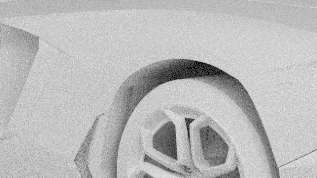
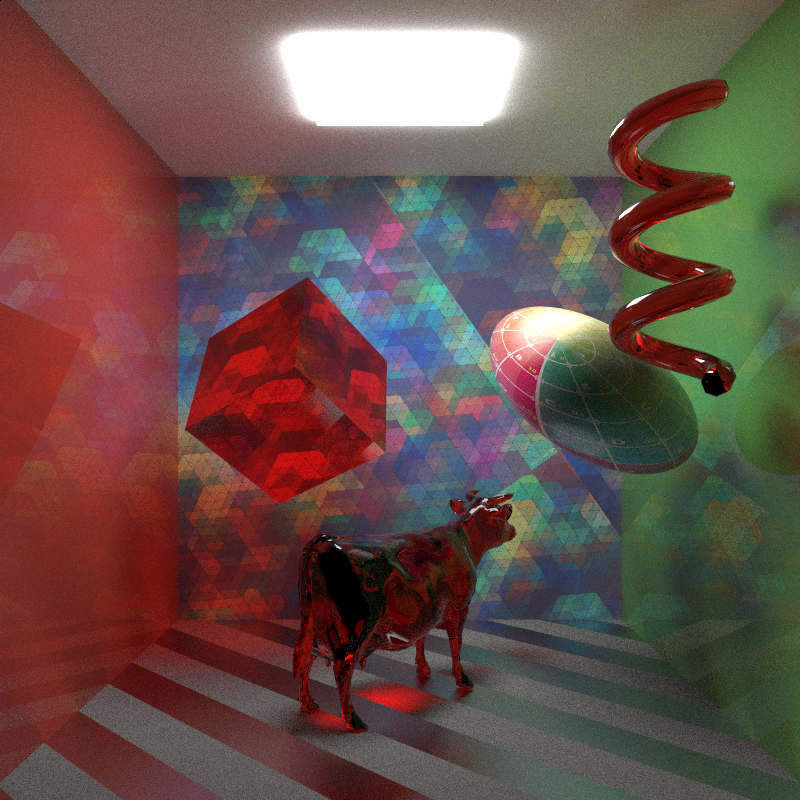
I went ahead and tried out this idea, and produced the following image:
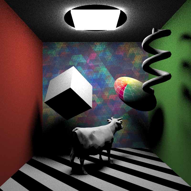
First off, for the most part, it works! The resulting direct illumination matches the ground truth and the BRDF-sampling render, but is significantly more converged than the BRDF-sampling render for the same number of samples. BUT, there is a critical flaw: note the black circle around the light source on the ceiling. That black circle happens to fall exactly within the bounding sphere for the light source, and results from a very simple mathematical fact: calculating the solid angle subtended by the bounding sphere for a point INSIDE of the bounding sphere is undefined. In other words, this shortcut approach will fail for any points that are too close to a light source.
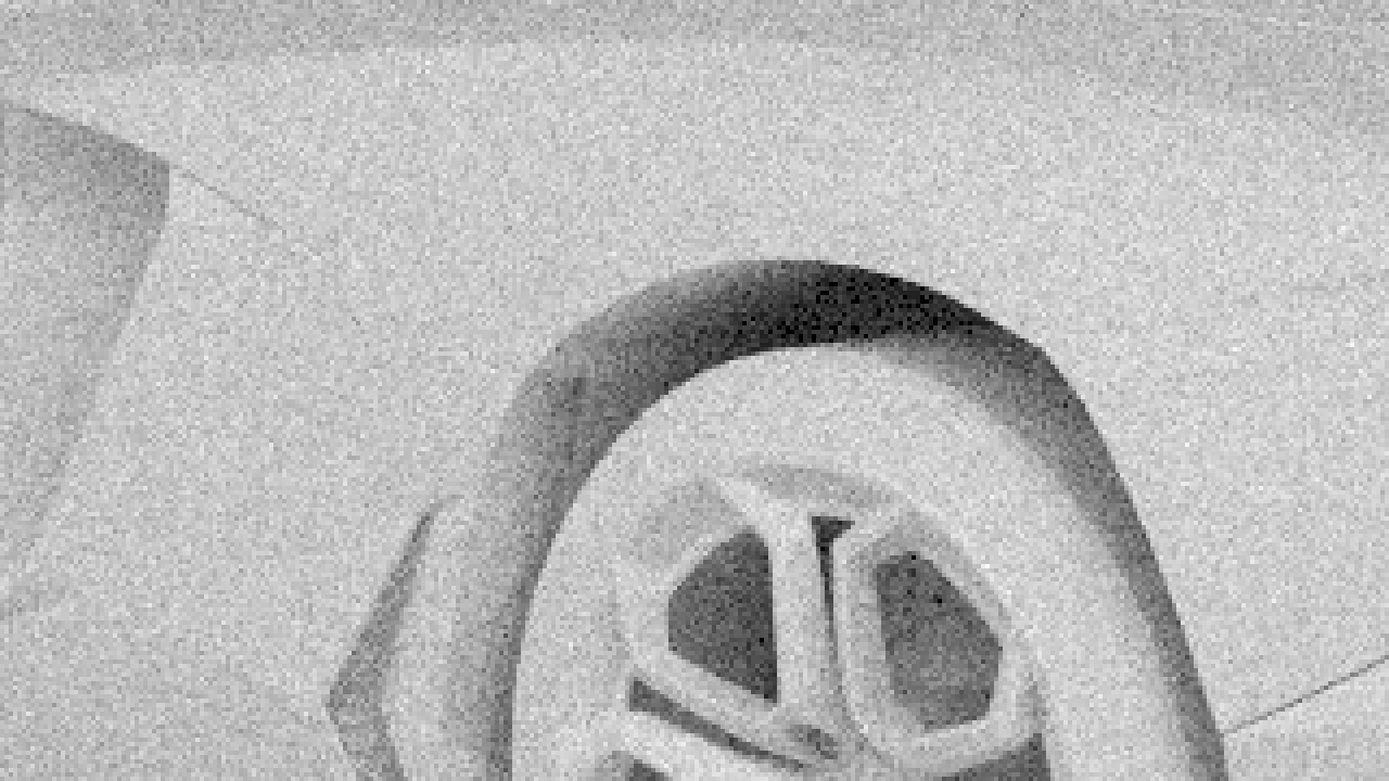
One possible workaround I tried was to have any points inside of a light’s bounding sphere to fall back to pure BRDF sampling, but this approach is also undesirable, as a highly visible discontinuity between the differently sampled area develops due to vastly different convergence rates.
So, while the overall solid angle weighting approach checks out, our shortcut does not. I’m now working on implementing the first approach described above, which should produce a correct result, and will post in the next few days.