Just a heads up, this post is admittedly more of a brain dump for myself than it is anything else.

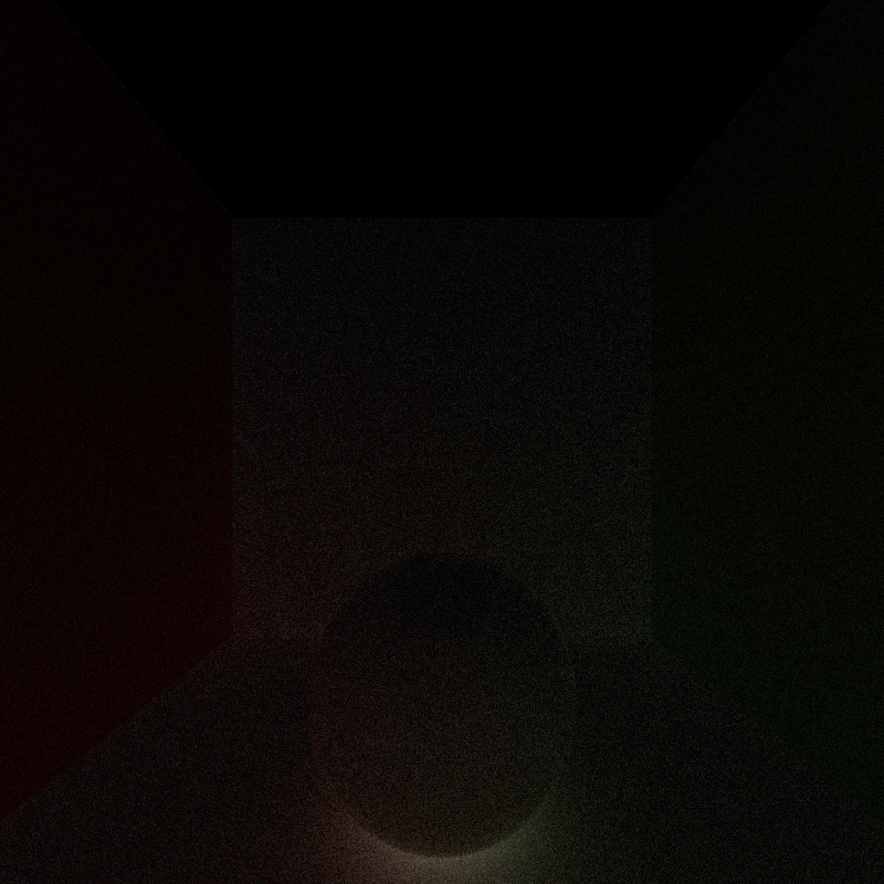
A while back I implemented a couple of fast methods to generate random points on geometry surfaces, which will be useful for a number of applications, such as direct lighting calculations involving area lights.

The way I’m sampling random points varies by geometry type, but all methods are pretty simple. Right now the system is implemented such that I can give the renderer a global point density to follow, and points will be generated according to that density value. This means the number of points generated on each piece of geometry is directly linked to the geometry’s surface area.

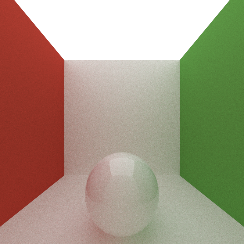
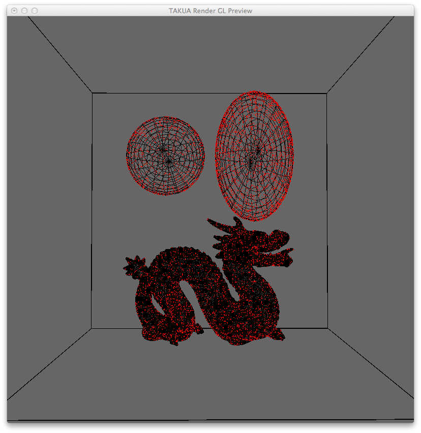
For spheres, the method I use is super simple: get the surface area of the sphere, generate random UV coordinates, and map those coordinates back to the surface of the sphere. This method is directly pulled from this Wolfram Mathworld page, which also describes why the most naive approach to point picking on a sphere is actually wrong.

My approach for ellipsoids unfortunately is a bit brute force. Since getting the actual surface area for an ellipsoid is actually fairly mathematically tricky, I just approximate it and then use plain old rejection sampling to get a point.

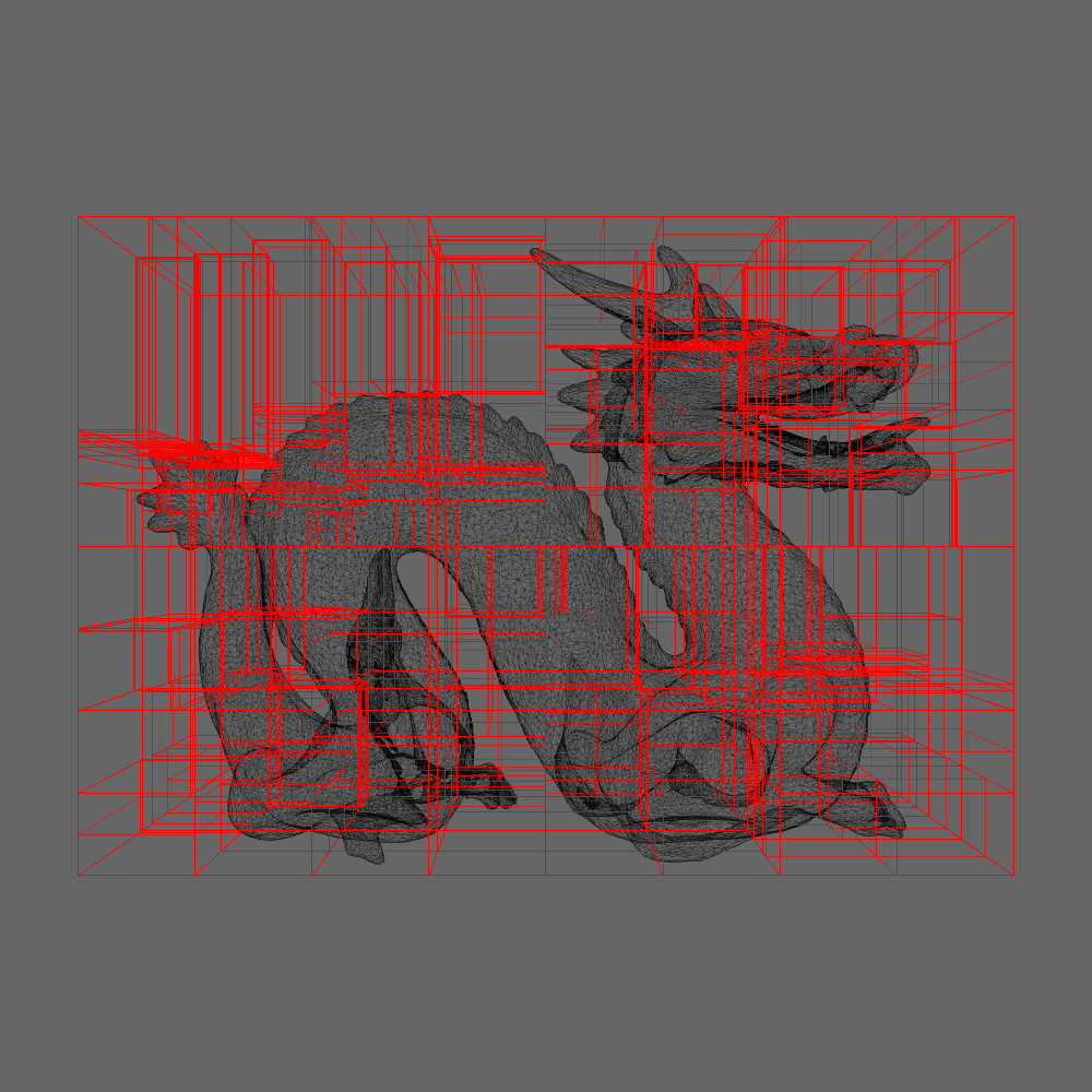
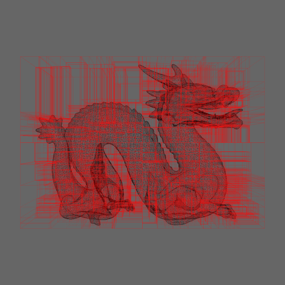
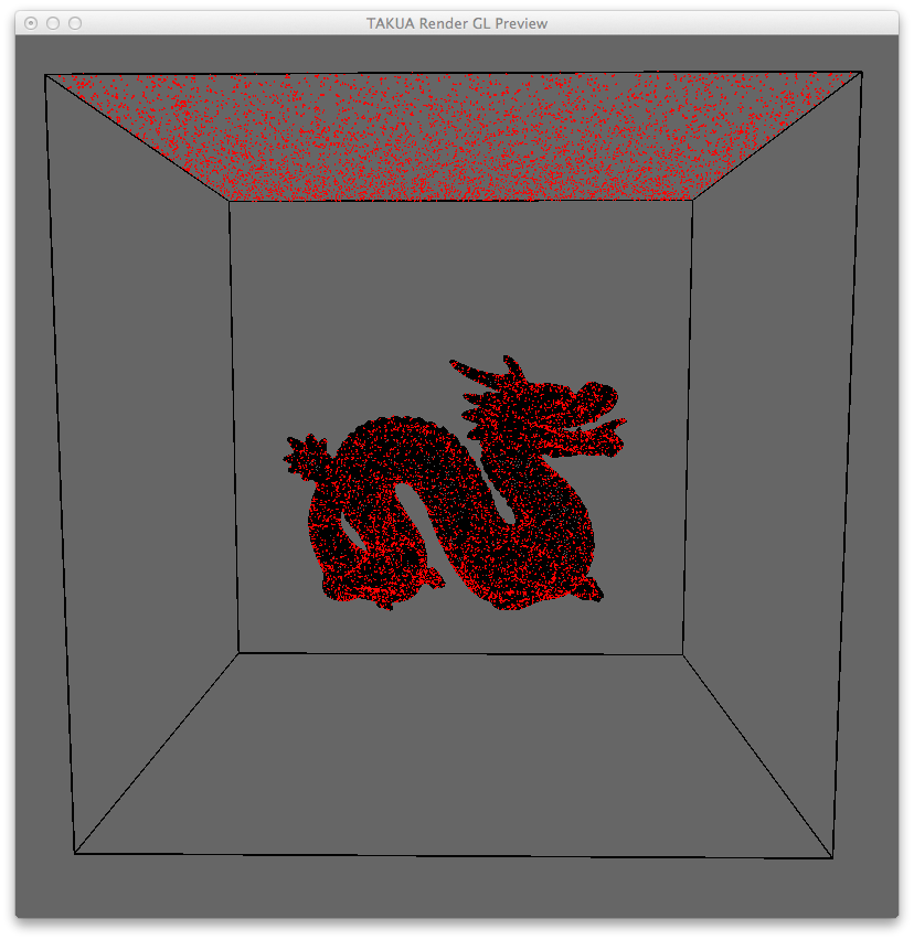
Boxes are the easiest of the bunch; find the surface area of each face, randomly select a face weighted by the proportion of the total surface area that face comprises, and then pick a random x and y coordinate on that face. The method I use for meshes is similar, just on potentially a larger scale: find the surface area of all of the faces in the mesh and select a face randomly weighted by the face’s proportion of the total surface area. Then instead of generating random cartesian coordinates, I generate a random barycentric coordinate, and I’m done.

The method that I’m using right now is purely random, so there’s no guarantee of equal spacing between points initially. Of course, as one picks more and more points, the spacing between any given set of points will converge on something like equally spaced, but that would take a lot of random points. I’ve been looking at this Dart Throwing On Surfaces Paper for ideas, but at least for now, this solution should work well enough for what I want it for (direct lighting). But we shall see!

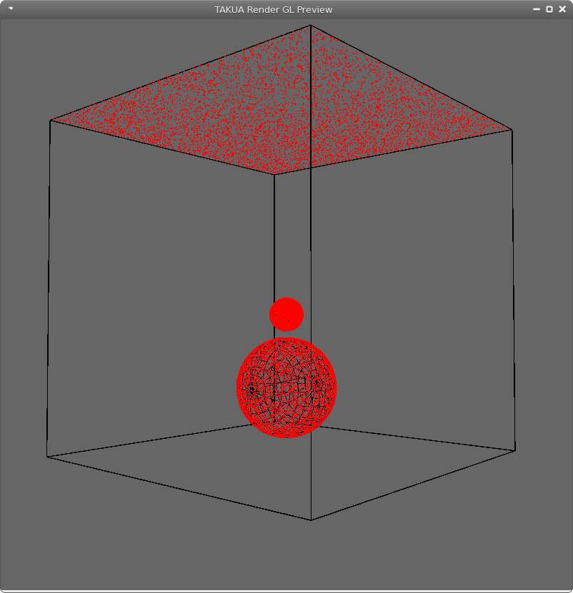
Also, as I am sure you can guess from the window chrome on that last screenshot, I’ve successfully tested Takua Render on Linux! Specifically, on Fedora!

I finally got around to doing a long overdue piece of analysis on Takua Render: looking at the impact of ray bounce depth on performance and on the final image.

Of course, in real life, light can bounce around (almost) indefinitely before it is either totally absorbed or enters our eyeballs. Unfortunately, simulating this behavior completely is extremely difficult in any type of raytracing solution because in a raytrace solution, letting a ray bounce around indefinitely until it does something interesting can lead to extremely extremely long render times. Thus, one of the first shortcuts that most raytracing (and therefore pathtracing) systems take is cutting off rays after they bounce a certain number of times. This strategy should not have much of an impact on the final visual quality of a rendered image, since the more a light ray bounces around, the less each successive bounce contributes to the final image anyway.

With that in mind, I did some tests with Takua Render in hopes of finding a good balance between ray bounce depth and quality/speed. The following images or a glossy white sphere in a Cornell Box were rendered on a quad-core 2.5 GhZ Core i5 machine.

For a reference, I started with a render with a maximum ray bounce depth of 50 and 200 samples per pixel:

Then I ran a test render with a maximum of just 2 bounces; essentially, this represents the direct lighting part of the solution only, albeit generated in a Monte Carlo fashion. Since I made the entire global limit 2 bounces, no reflections show up on the sphere of the walls, just the light overhead. Note the total lack of color bleeding and the dark shadow under the ball.

The next test was with a maximum of 5 bounces. In this test, nice effects like color bleeding and indirect illumination are back! However, compared to the reference render, the area under the sphere still has a bit of dark shadowing, much like what one would expect if an ambient occlusion pass had been added to the image. While not totally accurate to the reference render, this image under certain artistic guidelines might actually be acceptable, and renders considerably faster.

Differencing the 5 bounce render from the reference 50 bounce render shows that the 5 bounce one is ever so slightly dimmer and that most of the difference between the two images is in the shadow area under the sphere. Ignore the random fireflying pixels, which is just a result of standard pathtracing variance in the renders:

The next test was 10 bounces. At 10 bounces, the resultant images is essentially visually indistinguishable from the 50 bounce reference, as shown by the differenced image included. This result implies that beyond 10 bounces, the contributions of successive bounces to the final image are more or less negligible.

Finally, a test with a maximum of 20 bounces is still essentially indistinguishable from both the 10 bounce test and the 50 bounce reference:

Interestingly, render times do not scale linearly with maximum bounce depth! The reason for this relationship (or lack thereof) can be found in the fact that the longer a ray bounces around, the more likely it is to find a light source and terminate. At 20 bounces, the odds of a ray finding a light source is very very close to the odds of a ray finding a light source at 50 bounces, explaining the smallness of the gap in render time between 20 and 50 bounces (especially compared to the difference in render time between, say, 2 and 5 bounces).

Lately progress on my Takua Render project has slowed down a bit, since over this summer I am interning at Dreamworks Animation during weekdays. However, in the evenings and on weekends I am still been working at stuff!

Something that I never got around to doing for no particularly good reason was visualizing my KD-tree implementation. As such, I’ve known for a long time that my KD-tree is suboptimal, but have not actually been able to quickly determine to what degree my KD-tree is inefficient. However, since I now have a number of OpenGL based diagnostic views for Takua Render, I figured I no longer had a good excuse to not visualize my KD-tree. So last night I did just that! Here is what I got for the Stanford Dragon:

Just as I suspected, my KD-tree implementation was far from perfect. Some rough statistics I had my renderer output told me that even with the KD-tree, the renderer was still performing hundreds to even thousands of intersection tests against meshes. The above image explains why: each of those KD-tree leaf nodes are enormous, and therefore contain an enormous amount of objects!

Fortunately, after a bit of tinkering, I discovered that there’s nothing actually wrong with the KD-tree implementation itself. Instead, the sparseness of the tree is coming from how I tuned the tree building operation. With a bit of tinkering, I managed to get a fairly improved tree:

…and with a bit more of tuning and playing with maximum recursion depths:

Previously, my KD-tree construction routine based the construction on only a maximum recursion depth; after the tree reached a certain height, the construction would stop. I’ve now modified the construction routine to use three separate criteria: a maximum recursion depth, minimum node bounding box volume, and a minimum number of objects per node. If any node meets any of the above three conditions, it is turned into a leaf node. As a result, I can now get extremely dense KD-trees that only have on average a low-single-digit number of objects per leaf node, as opposed to the average hundreds of objects per leaf node before:

In theory, this improvement should allow for a fairly significant speedup, since the number of intersections per mesh should now be dramatically lower, leading to much higher ray throughput! I’m currently running some benchmarks to determine just how much of a performance boost better KD-trees will give me, and I’ll post about those results soon!

I implemented subsurface scattering in my renderer!

Here’s a Stanford Dragon in a totally empty environment with just one light source providing illumination. The dragon is made up of a translucent purple jelly-like material, showing off the subsurface scattering effect:

Subsurface scattering is an important behavior that light exhibits upon hitting some translucent materials; normal transmissive materials will simply transport light through the material and out the other side, but subsurface scattering materials will attenuate and scatter light before releasing the light somewhere not necessarily along a line from the entry point. This is what gives skin and translucent fruit and marble and a whole host of other materials their distinctive look.

There are currently a whole host of methods to rapidly approximate subsurface scattering, including some screen-space techniques that are actually fast enough for use in realtime renderers. However, my implementation at the moment is purely brute-force monte-carlo; while extremely physically accurate, it is also very very slow. In my implementation, when a ray enters a subsurface scattering material, I generate a random scatter direction via isotropic scattering, and then calculate light accumulation attenuation based on an absorption coefficient defined for the material. This approach is very similar to the one taken by Peter and me in our GPU pathtracer.

At some point in the future I might try out a faster approximation method, but for the time being, I’m pretty happy with the visual result that brute-force monte-carlo scattering produces.

Here’s the same subsurface scattering dragon from above, but now in the Cornell Box. Note the cool colored soft shadows beneath the dragon:

Also, I’ve finally settled on a name for my renderer project: Takua Render! So, that is what I shall be calling my renderer from now on!