One question I’ve been asking myself ever since my friend Peter Kutz and I wrapped our little GPU Pathtracer experiment is “why am I writing Takua Renderer as a CPU-only renderer?” One of the biggest lessons learned from the GPU Pathtracer experiment was that GPUs can indeed provide vast quantities of compute suitable for use in pathtracing rendering. After thinking for a bit at the beginning of the summer, I’ve decided that since I’m starting my renderer from scratch and don’t have to worry about the tons of legacy that real-world big boy renderers like RenderMan have to deal with, there is no reason why I shouldn’t architect my renderer to use whatever compute power is available.

With that being said, from this point forward, I will be concurrently developing CPU and GPU based implementations of Takua Renderer. I call this new overall project TAKUA/Avohkii, mainly because Avohkii is a cool name. Within this project, I will continue developing the C++ based x86 version of Takua, which will retain the name of just Takua, and I will also work on a CUDA based GPU version, called Takua-RT, with full feature parity. I’m also planning on investigating the idea of an ARM port, but that’s an idea for later. I’m going to stick with CUDA for the GPU version now since I know CUDA better than OpenCL and since almost all of the hardware I have access to develop and test on right now is NVIDIA based (the SIG Lab runs on NVIDIA cards…), but that could change down the line. The eventual goal is to have a set of renderers that together cover as many hardware bases as possible, and can all interoperate and intercommunicate for farming purposes.

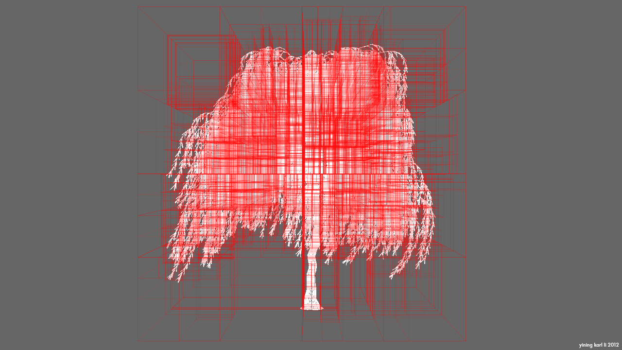
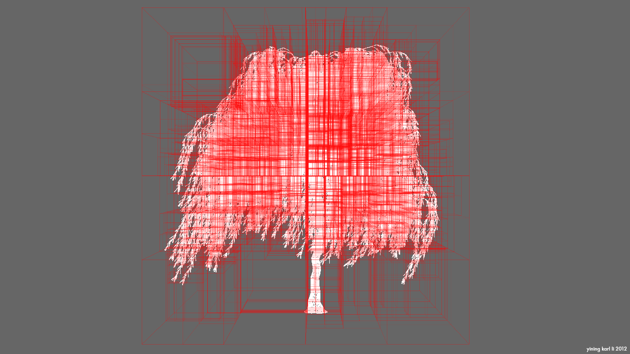
I’ve already gone ahead and finished the initial work of porting Takua Renderer to CUDA. One major lesson learned from the GPU Pathtracer experiment was that enormous CUDA kernels tend to run into a number of problems, much like massive monolithic GL shaders do. One problem in particular is that enormous kernels tend to take a long time to run and can result in the GPU driver terminating the kernel, since NVIDIA’s drivers by default assume that device threads taking longer than 2 seconds to run are hanging and cull said threads. In the GPU Pathtracer experiment, we used a giant monolithic kernel for a single ray bounce, which ran into problems as geometry count went up and subsequently intersection testing and therefore kernel execution time also increased. For Takua-RT, I’ve decided to split a single ray bounce into a sequence of micro-kernels that launch in succession. Basically, each operation is now a kernel; each intersection test is a kernel, BRDF evaluation is a kernel, etc. While I suppose I lose a bit of time in having numerous kernel launches, I am getting around the kernel time-out problem.

Another important lesson learned was that culling useless kernel launches is extremely important. I’m checking for empty threads at the end of each ray bounce and culling via string compaction for now, but this can of course be further extended to the micro-kernels for intersection testing later.

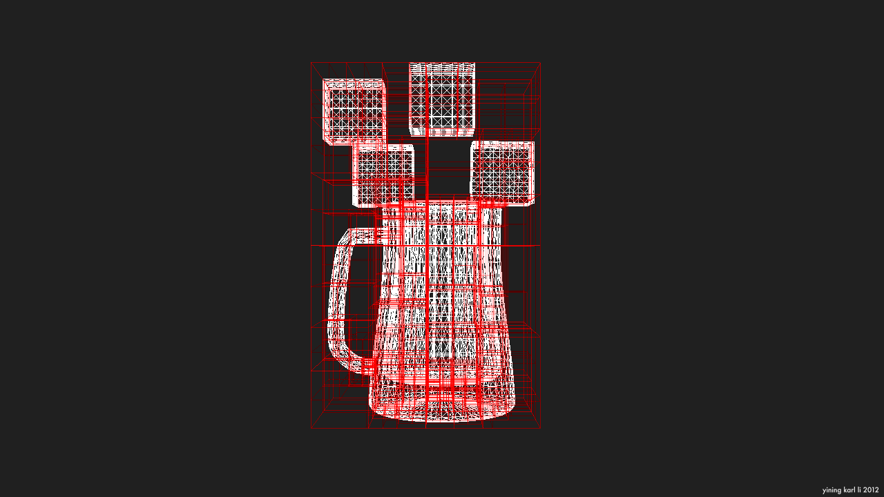
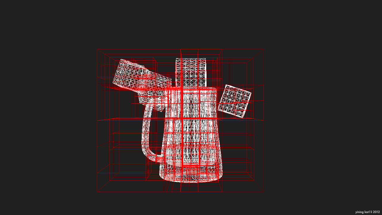
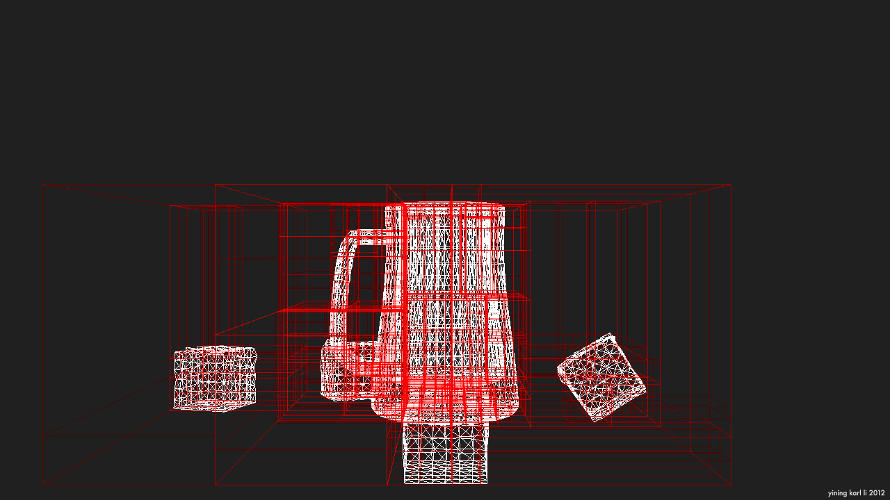
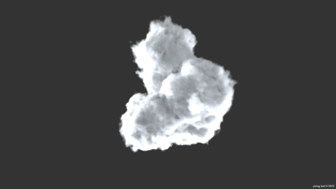
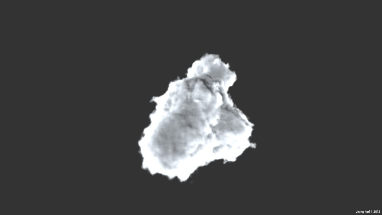
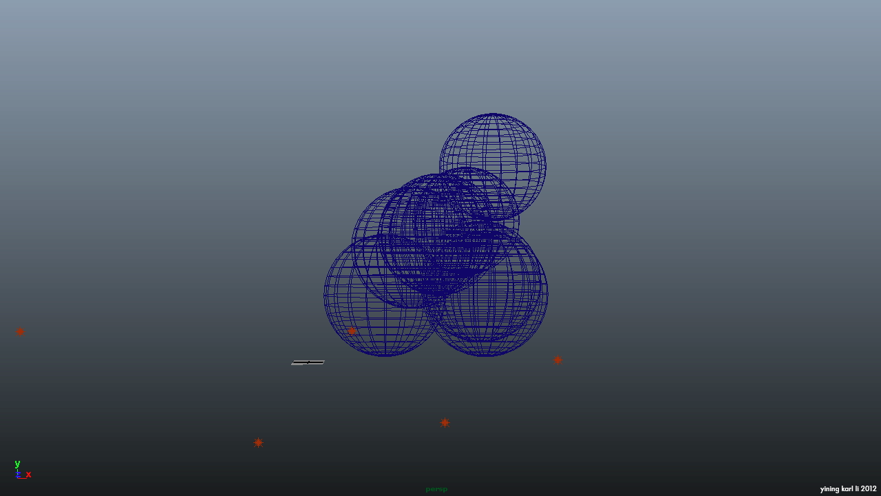
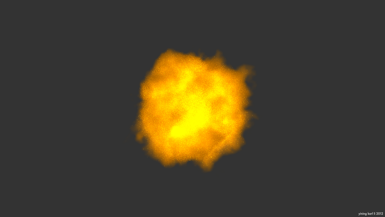
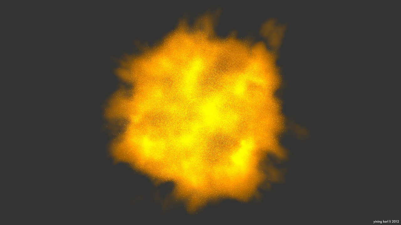
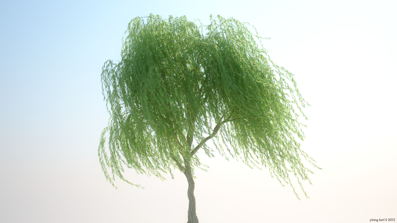
Anyhow, enough text. Takua-RT, even in its super-naive unoptimized CUDA-port state right now, is already so much faster than the CPU version that I can render frames with fairly high convergence in seconds to minutes. That means the renderer is now fast enough for use on rendering animations, such as the one at the top of this post. No post-processing whatsoever was applied, aside from my name watermark in the lower right hand corner. The following images are raw output frames from Takua-RT, this time straight from the renderer, without even watermarking:

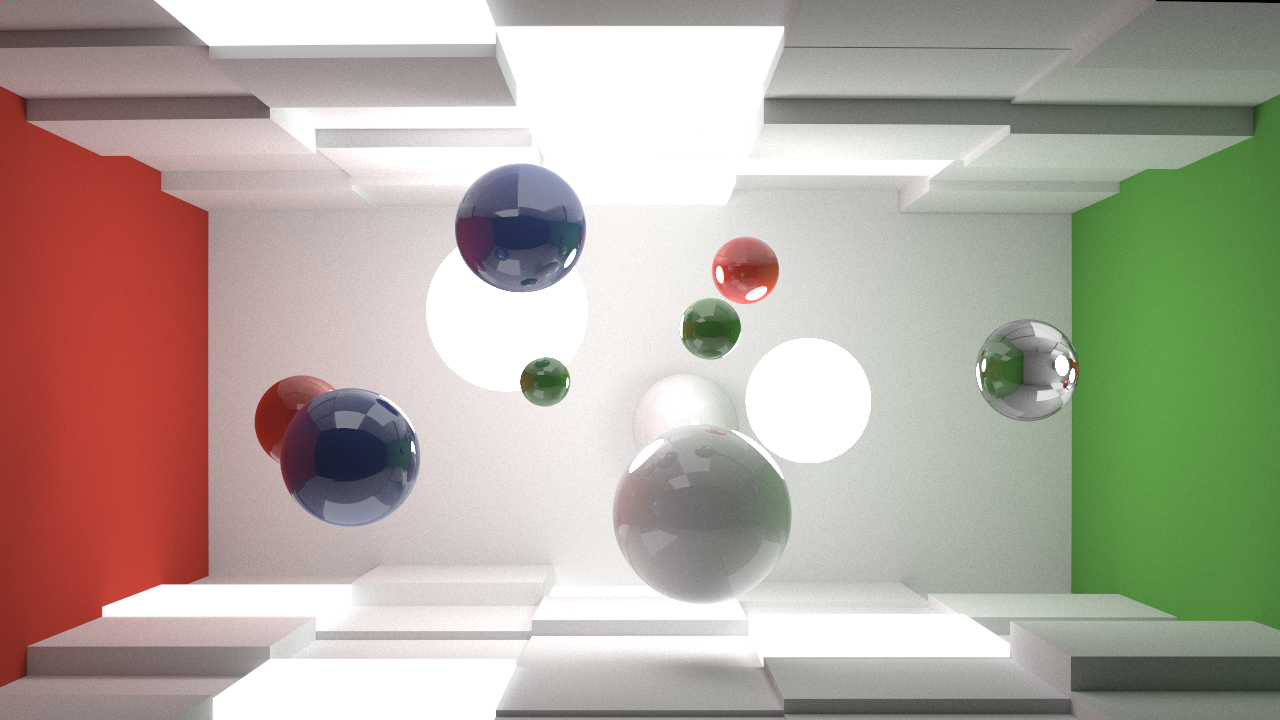
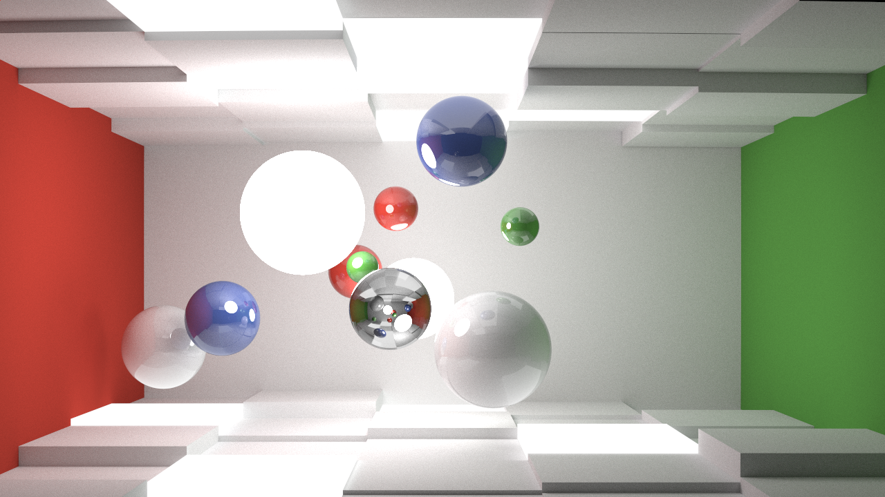
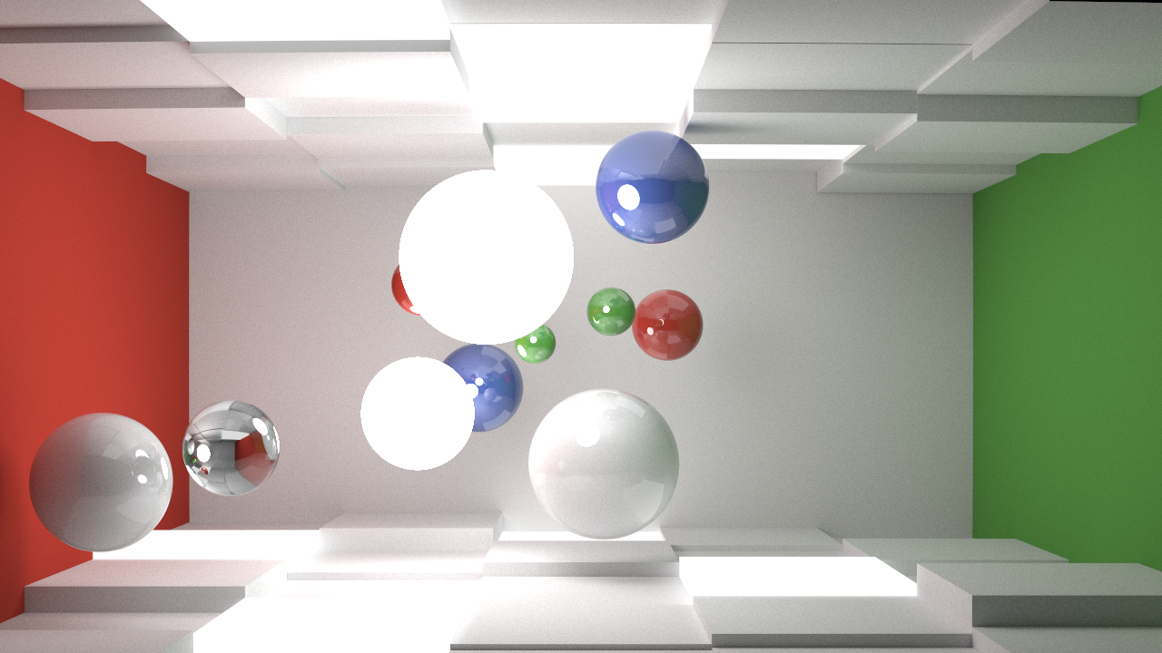
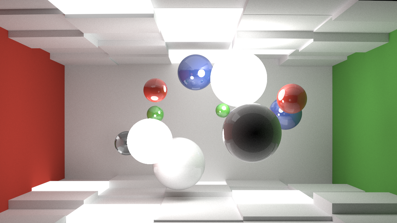
Each of these frames represents 5000 iterations of convergence, and took about a minute to render on a NVIDIA Geforce GTX480. The flickering in the glass ball in animated version comes from having a low trace depth of 3 bounces, including for glass surfaces.

I’ve started an effort to clean up, rewrite, and enhance my ObjCore library, and part of that effort includes taking my KD-Tree viewer from Takua Render and making it just a standard component of ObjCore. As a result, I can now plug the latest version of ObjCore into any of my projects that use it and quickly wire up support for viewing the KD-Tree view for that project. Here’s the jello sim from a few months back visualized as a KD-Tree:

I’ve adopted a new standard grey background for OpenGL tests, since I’ve found that the higher amount of contrast this darker grey provides plays nicer with Vimeo’s compression for a clearer result. But of course I’ll still post stills too.

Hopefully at the end of this clean up process, I’ll have ObjCore in a solid enough of a state to post to Github.

I’ve been meaning to add animation support to my volume renderer for demoreel purposes for a while now, so I did that this week! Here’s a rotating cloud animation:

…and of course, a still or two:

Instead of just rotating the camera around the cloud, I wanted for the cloud itself to rotate but have the noise field it samples stay stationary, resulting in a cool kind of morphing effect with the cloud’s actual shape. In order to author animations easily, I implemented a fairly rough, crude version of Maya integration. I wrote a script that will take spheres and point lights in Maya and build a scene file for my volume renderer using the Maya spheres to define cloud clusters and the point lights to define… well… lights. With an easy bit of scripting, I can do this for each frame in a keyframed animation in Maya and then simply call the volume renderer once for each frame. Here’s what the above animation’s Maya scene file looks like:

Also, since my pseudo-blackbody trick was originally intended to simulate the appearance of a fireball, I tried creating an animation of a fireball by just scaling a sphere:

…and as usual again, stills:

So that’s that for the volume renderer for now! I think this might be the end of the line for this particular incarnation of the volume renderer (it remains the only piece of tech I’m keeping around that is more or less unmodified from its original CIS460/560 state). I think the next time I revisit the volume renderer, I’m either going to port it entirely to CUDA, as my good friend Adam Mally did with his, or I’m going to integrate it into my renderer project, Peter Kutz style.

Every once in a while, I return to trying to make a good looking tree. Here’s a frame from my latest attempt:

Have I finally managed to create a tree that I’m happy with? Well….. no. But I do think this batch comes closer than previous attempts! I’ve had a workflow for creating base tree geometry for a while now that I’m fairly pleased with, which is centered around using OnyxTREE as a starting point and then custom sculpting in Maya and Mudbox. However, I haven’t tried actually animating trees before, and shading trees properly has remained a challenge. So, my goal this time around was to see if I could make any progress in animating and shading trees.

As a starting point, I played with just using the built in wind simulation tools in OnyxTREE, which was admittedly difficult to control. I found that having medium to high windspeeds usually led to random branches glitching out and jumping all over the place. I also wanted to make a weeping willow style tree, and even medium-low windspeeds often resulted in the hilarious results:

A bigger problem though was the sheer amount of storage space exporting animated tree sequences from Onyx to Maya requires. The only way to bring Onyx simulations into programs that aren’t 3ds Max is to export the simulation as an obj sequence from Onyx and then import the sequence into whatever program. Maya doesn’t have a native method to import obj sequences, so I wrote a custom Python script to take care of it for me. Here’s a short compilation of some results:

One important thing I discovered was that the vertex numbering in each obj frame exported from Onyx remains consistent; this fact allowed for an important improvement. Instead of storing a gazillion individual frames of obj meshes, I experimented with dropping a large number of intermediate frames and leaving a relatively smaller number of keyframes which I then used as blendshape frames with more scripting hackery. This method works rather well; in the above video, the weeping willow at the end uses this approach. There is, however, a significant flaw with this entire Onyx based animation workflow: geometry clipping. Onyx’s system does not resolve cases where leaves and entire branches clip through each other… while from a distance the trees look fine, up close the clipping can become quite apparent. For this reason, I’m thinking about abandoning the Onyx approach altogether down the line and perhaps experimenting with building my own tree rigs and procedurally animating them. That’s a project for another day, however.

On the shading front, my basic approach is still the same: use a Vray double sided material with a waxier, more specular shader for the “front” of the leaves and a more diffuse shader for the “back”. In real life, leaves of course display an enormous amount of subsurface scattering, but leaves are a special case for subsurface scatter: they’re really really thin! Normally subsurface scattering is a rather expensive effect to render, but for thin material cases, the Vray double sided material can quite efficiently approximate the subsurface effect for a fraction of the rendertime.

Bark is fairly straightforward to, it all comes down to the displacement and bump mapping. Unfortunately, the limbs in the tree models I made this time around were straight because I forgot to go in and vary them up/sculpt them. Because of the straightness, my tree twigs don’t look very good this time, even with a decent shader. Must remember for next time! Creating displacement bark maps from photographs or images sourced from Google Image Search or whatever is really simple; take your color texture into Photoshop, slam it to black and white, and adjust contrast as necessary:

Here’s a few seconds of rendered output with the camera inside of the tree’s leaf canopy, pointed skyward. It’s not exactly totally realistic looking, meaning it needs more work of course, but I do like the green-ess of the whole thing. More importantly, you can see the subsurface effect on the leaves from the double sided material!

Something that continues to prove challenging is how my shaders hold up at various distances. The same exact shader (with a different leaf texture), looks great from a distance, but loses realism when the camera is closer. I did a test render of the weeping willow from further away using the same shader, and it looks a lot better. Still not perfect, but closer than previous attempts:

…and of course, a pretty still or two:

A fun experiment I tried was building a shader that can imitate the color change that occurs as fall comes around. This shader is in no way physically based, it’s using just a pure mix function controlled through keyframes. Here’s a quick test showing the result:

Eventually building a physically based leaf BSSDF system might be a fun project for my own renderer. Speaking of which, I couldn’t resist throwing the weeping willow model through my KD-tree library to get a tree KD-tree:

Since the Vimeo compression kind of borks thin lines, here’s a few stills:

Alright, that’s all for this time! I will most likely return to trees yet again perhaps a few weeks or months from now, but for now, much has been learned!