This year at SIGGRAPH 2019, Matt Jen-Yuan Chiang, Brent Burley, and I had a talk that presents a technique for smoothing out the harsh shadow terminator problem that often arises when high-frequency bump or normal mapping is used in ray tracing. We developed this technique as part general development on Disney’s Hyperion Renderer for the production of Frozen 2. This work is mostly Matt’s; Matt was very kind in allowing me to help out and play a small role on this project.

This work is contemporaneous with the recent work on the same shadow terminator problem that was carried out and published by Estevez et al. from Sony Pictures Imageworks and published in Ray Tracing Gems. We actually found out about the Estevez et al. technique at almost exactly the same time that we submitted our SIGGRAPH talk, which proved to be very fortunate, since after our talk was accepted, we were than able to update our short paper with additional comparisons between Estevez et al. and our technique. I think this is a great example of how having multiple rendering teams in the field tackling similar problems and sharing results provides a huge benefit to the field as a whole- we now have two different, really good solutions to what used to be a big shading problem!

Here is the paper abstract:

A longstanding problem with the use of shading normals is the discontinuity introduced into the cosine falloff where part of the hemisphere around the shading normal falls below the geometric surface. Our solution is to add a geometrically derived shadowing function that adds minimal additional shadowing while falling smoothly to zero at the terminator. Our shadowing function is simple, robust, efficient and production proven.

The paper and related materials can be found at:

• Project Page (Author’s Version and Presentation Slides)
• Official Print Version (ACM Library)

Matt Chiang presented the paper at SIGGRAPH 2019 in Los Angeles as part of the “Lucy in the Sky with Diamonds - Processing Visuals” Talks session. A pdf version of the presentation slides, along with presenter notes, are available on my project page for the paper. I’d also recommend getting the author’s version of the short paper instead of the official version as well, since the author’s version includes some typo fixes made after the official version was published.

Work on this project started early in the production of Frozen 2, when our look artists started to develop the shading of the dresses and costumes in Frozen 2. Because intricate woven fabrics and patterns are an important part of the Scandinavian culture that Frozen 2 is inspired by, the shading in Frozen 2 pushed high-resolution high-frequency displacing and normal mapping further than we ever had before with Hyperion in order to make convincing looking textiles. Because of how high-frequency the normal mapping was pushed, the bump/normal mapped shadow terminator problem became worse and worse and proved to be a major pain point for our look and lighting artists. In the past, our look and lighting artists have worked around shadow terminator issues using a combination of techniques, such as falling back to full displacement, or using larger area lights to try to soften the shadow terminator. However, these techniques can be problematic when they are in conflict with art direction, and force artists to think about an additional technical dimension when they otherwise would rather be focused on the artistry.

Our search for a solution began with Peter Kutz looking at “Microfacet-based Normal Mapping for Robust Monte Carlo Path Tracing” by Schüssler et al., which focused on addressing energy loss when rendering shading normals. The Schüssler et al. 2017 technique solved the energy loss problem by constructing a microfacet surface comprised of two facets per shading point, instead the the usual one. The secondary facet is used to account for things like inter-reflections between the primary and secondary facets. However, the Schüssler et al. 2017 technique wound up not solving the shadow terminator problems we were facing; using their shadowing function produced a look that was too flat.

Matt Chiang then realized that the secondary microfacet approach could be used to solve the shadow terminator problem using a different secondary microfacet configuration; instead of using a vertical second facet as in Schüssler, Matt made the secondary facet perpendicular to the shading normal. By making the secondary facet perpendicular, as a light source slowly moves towards the grazing angle relative to the microfacet surface, peak brightness is maintained when the light is parallel to the shading normal, while additional shadowing is introduced beyond the parallel angle. This solution worked extremely well, and is the technique presented in our talk / short paper.

The final piece of the puzzle was addressing a visual discontinuity produced by Matt’s technique when the light direction reaches and moves beyond the shading normal. Instead of falling smoothly to zero, the shape of the shadow terminator undergoes a hard shift from a cosing fall-off formed by the dot product of the shading normal and light direction to a linear fall-off. Matt and I played with a number of different interpolation schemes to smooth out this transition, and eventually settled on a custom smooth-step function. During this process, I made the observation that whatever blending function we used needed to introduce C1 continuity in order to remove the visual discontinuity. This observation led Brent Burley to realize that instead of a complex custom smooth-step function, a simple Hermite interpolation would be enough; this Hermite interpolation is the one presented in the talk / short paper.

For a much more in-depth view at all of the above, complete with diagrams and figures and examples, I highly recommend looking at Matt’s presentation slides and presenter notes.

Here is a test render of the Iduna character’s costume from Frozen 2, from before we had this technique implemented in Hyperion. The harsh shadow terminator produces an illusion that makes her arms and torso look boxier than the actual underlying geometry is:

…and here is the same test render, but now with our soft shadow terminator fix implemented and enabled. Note how her arms and torso now look properly rounded, instead of boxy!

This technique is now enabled by default across the board in Hyperion, and any article of clothing or costume you see in Frozen 2 is using this technique. So, through this project, we got to play a small role in making Elsa, Anna, Kristoff, and everyone else look like themselves!

Table of Contents

Introduction

Every year at SIGGRAPH (and sometimes at other points in the year), members of the Hyperion team inevitably get asked if there is any publicly available information about Disney’s Hyperion Renderer. The answer is: yes, there is actually a lot of publicly available information!

One amazing aspect of working at Walt Disney Animation Studios is the huge amount of support and encouragement we get from our managers and the wider studio for publishing and sharing our work with the wider academic world and industry. As part of this sharing, the Hyperion team has had the opportunity to publish a number of papers over the years detailing various interesting techniques used in the renderer.

I think it’s very important to mention here that another one of my favorite aspects of working on the Hyperion team is the deep collaboration we get to engage in with our sister rendering team at DisneyResearch|Studios (formerly known as Disney Research Zürich). The vast majority of the Hyperion team’s publications are joint works with DisneyResearch|Studios, and I personally think it’s fair to say that all of Hyperion’s most interesting advanced features are just as much the result of research and work from DisneyResearch|Studios as they are the result of our team’s own work. Without a doubt, Hyperion, and by extension, our movies, would not be what they are today without DisneyResearch|Studios. Of course, we also collaborate closely with our sister rendering teams at Pixar Animation Studios and Industrial Light & Magic as well, and there are numerous examples where collaboration between all of these teams has advanced the state of the art in rendering for the whole industry.

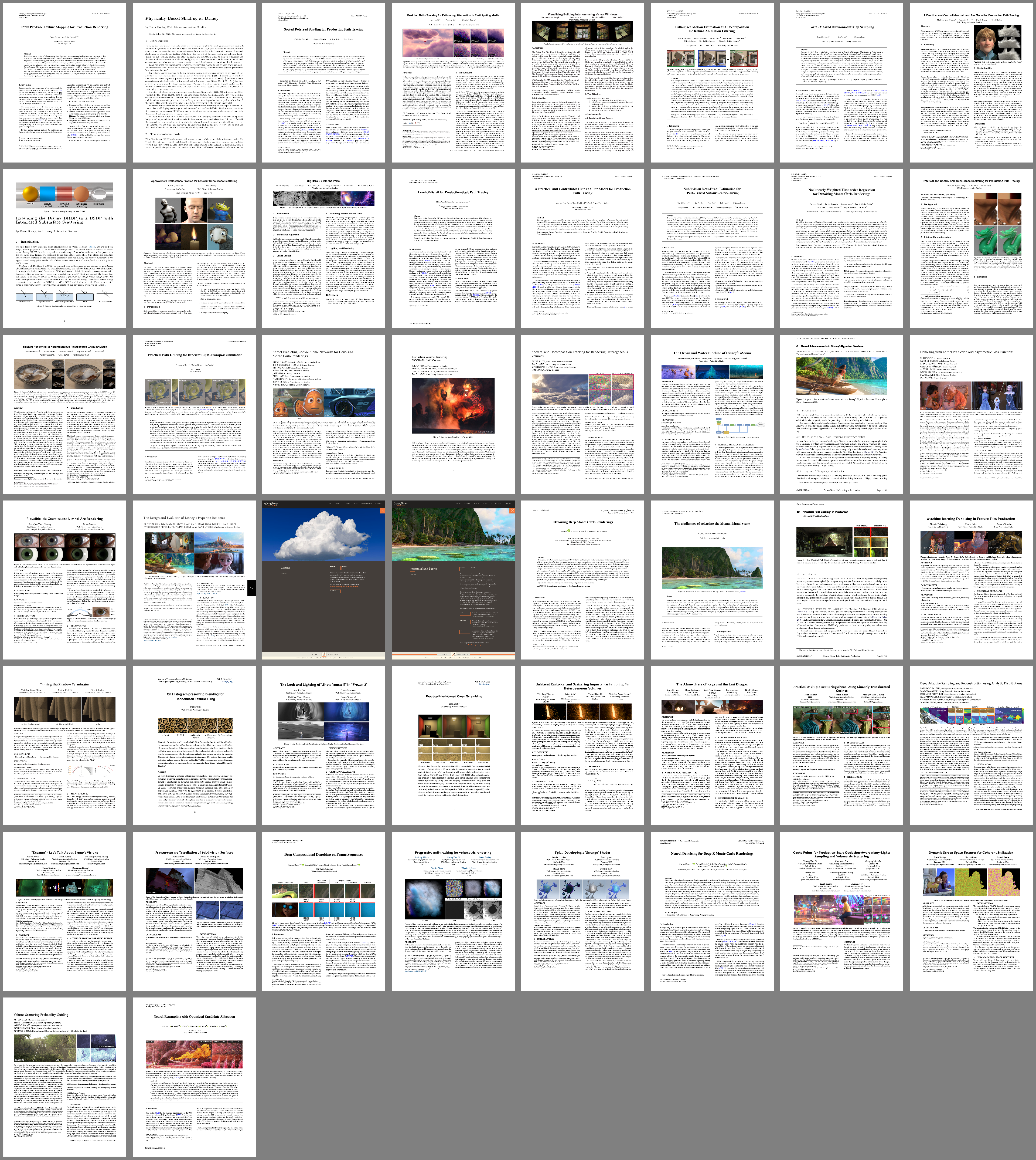
So without further ado, below are all of the papers that the Hyperion team has published or worked on or had involvement with over the years, either by ourselves or with our counterparts at DisneyResearch|Studios, Pixar, ILM, and other research groups. If you’ve ever been curious to learn more about Disney’s Hyperion Renderer, here are 52 publications with a combined 571 pages of material! For each paper, I’ll link to a preprint version, link to the official publisher’s version, and link any additional relevant resources for the paper. Please see publisher’s version or project page links for any additional supplemental materials that go with each paper. I’ll also give the citation information, give a brief description, list the teams involved, and note how the paper is relevant to Hyperion. This post is meant to be a living document; I’ll come back and update it down the line with future publications. Publications are listed in chronological order.

Publications

1. Ptex: Per-Face Texture Mapping for Production Rendering

   Brent Burley and Dylan Lacewell. Ptex: Per-face Texture Mapping for Production Rendering. Computer Graphics Forum (Proceedings of Eurographics Symposium on Rendering 2008), 27(4), June 2008.

   • Preprint Version
   • Official Publisher’s Version
   • Open Source Project

   Internal project from Disney Animation. This paper describes per-face textures, a UV-free way of texture mapping. Ptex is the texturing system used in Hyperion for all non-procedural texture maps. Every Disney Animation film made using Hyperion is textured entirely with Ptex. Ptex is also available in many commercial renderers, such as Pixar’s RenderMan!

2. Physically-Based Shading at Disney

   Brent Burley. Physically Based Shading at Disney. In ACM SIGGRAPH 2012 Course Notes: Practical Physically-Based Shading in Film and Game Production, August 2012.

   • Preprint Version (Updated compared to official version)
   • Official Publisher’s Version
   • Physically Based Shading SIGGRAPH 2012 Course

   Internal project from Disney Animation. This paper describes the Disney BRDF, a physically principled shading model with a artist-friendly parameterization and layering system. The Disney BRDF is the basis of Hyperion’s entire shading system. The Disney BRDF has also gained widespread industry adoption the basis of a wide variety of physically based shading systems, and has influenced the design of shading systems in a number of other production renderers. Every Disney Animation film made using Hyperion is shaded using the Disney BSDF (an extended version of the Disney BRDF, described in a later paper).

3. Sorted Deferred Shading for Production Path Tracing

   Christian Eisenacher, Gregory Nichols, Andrew Selle, and Brent Burley. Sorted Deferred Shading for Production Path Tracing. Computer Graphics Forum (Proceedings of Eurographics Symposium on Rendering 2013), 32(4), June 2013.

   • Preprint Version
   • Official Publisher’s Version

   Internal project from Disney Animation. Won the Best Paper Award at EGSR 2013! This paper describes the sorted deferred shading architecture that is at the very core of Hyperion. Along with the previous two papers in this list, this is one of the foundational papers for Hyperion; every film rendered using Hyperion is rendered using this architecture.

4. Residual Ratio Tracking for Estimating Attenuation in Participating Media

   Jan Novák, Andrew Selle, and Wojciech Jarosz. Residual Ratio Tracking for Estimating Attenuation in Participating Media. ACM Transactions on Graphics (Proceedings of SIGGRAPH Asia 2014), 33(6), November 2014.

   • Preprint Version
   • Official Publisher’s Version
   • Project Page

   Joint project between DisneyResearch|Studios and Disney Animation. This paper described a pair of new, complementary techniques for evaluating transmittance in heterogeneous volumes. These two techniques made up the core of Hyperion’s first and second generation volume rendering implementations, used from Big Hero 6 up through Moana.

5. Visualizing Building Interiors using Virtual Windows

   Norman Moses Joseph, Brett Achorn, Sean D. Jenkins, and Hank Driskill. Visualizing Building Interiors using Virtual Windows. In ACM SIGGRAPH Asia 2014 Technical Briefs, December 2014.

   • Preprint Version
   • Official Publisher’s Version

   Internal project from Disney Animation. This paper describes Hyperion’s “hologram shader”, which is used for creating the appearance of parallaxed, fully shaded, detailed building interiors without adding additional geometric complexity to a scene. This technique was developed for Big Hero 6. Be sure to check out the supplemental materials on the publisher site for a cool video breakdown of the technique.

6. Path-space Motion Estimation and Decomposition for Robust Animation Filtering

   Henning Zimmer, Fabrice Rousselle, Wenzel Jakob, Oliver Wang, David Adler, Wojciech Jarosz, Olga Sorkine-Hornung, and Alexander Sorkine-Hornung. Path-space Motion Estimation and Decomposition for Robust Animation Filtering. Computer Graphics Forum (Proceedings of Eurographics Symposium on Rendering 2015), 34(4), June 2015.

   • Preprint Version
   • Official Publisher’s Version
   • Project Page

   Joint project between DisneyResearch|Studios, ETH Zürich, and Disney Animation. This paper describes a denoising technique suitable for animated sequences. Not directly used in Hyperion’s denoiser, but both inspired by and influential towards Hyperion’s first generation denoiser.

7. Portal-Masked Environment Map Sampling

   Benedikt Bitterli, Jan Novák, and Wojciech Jarosz. Portal-Masked Environment Map Sampling. Computer Graphics Forum (Proceedings of Eurographics Symposium on Rendering 2015), 34(4), June 2015.

   • Preprint Version
   • Official Publisher’s Version
   • Project Page

   Joint project between DisneyResearch|Studios and Disney Animation. This paper describes an efficient method for importance sampling environment maps. This paper was actually derived from the technique Hyperion uses for importance sampling lights with IES profiles, which has been used on all films rendered using Hyperion.

8. A Practical and Controllable Hair and Fur Model for Production Path Tracing

   Matt Jen-Yuan Chiang, Benedikt Bitterli, Chuck Tappan, and Brent Burley. A Practical and Controllable Hair and Fur Model for Production Path Tracing. In ACM SIGGRAPH 2015 Talks, August 2015.

   • Preprint Version
   • Official Publisher’s Version

   Joint project between DisneyResearch|Studios and Disney Animation. This short paper gives an overview of Hyperion’s fur and hair model, originally developed for use on Zootopia. A full paper was published later with more details. This fur/hair model is Hyperion’s fur/hair model today, used on every film beginning with Zootopia to present.

9. Extending the Disney BRDF to a BSDF with Integrated Subsurface Scattering

   Brent Burley. Extending the Disney BRDF to a BSDF with Integrated Subsurface Scattering. In ACM SIGGRAPH 2015 Course Notes: Physically Based Shading in Theory and Practice, August 2015.

   • Preprint Version
   • Official Publisher’s Version
   • Physically Based Shading SIGGRAPH 2015 Course

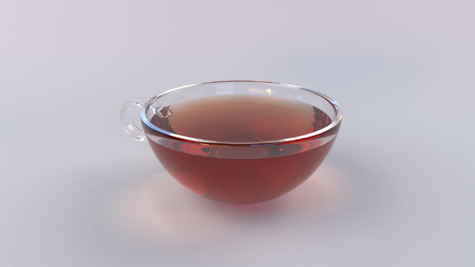
   Internal project from Disney Animation. This paper describes the full Disney BSDF (sometimes referred to in the wider industry as Disney BRDF v2) used in Hyperion, and also describes a novel subsurface scattering technique called normalized diffusion subsurface scattering. The Disney BSDF is the shading model for everything ever rendered using Hyperion, and normalized diffusion was Hyperion’s subsurface model from Big Hero 6 up through Moana. For a public open-source implementation of the Disney BSDF, check out PBRT v3’s implementation. Also, check out Pixar’s RenderMan for an implementation in a commercial renderer!

10. Approximate Reflectance Profiles for Efficient Subsurface Scattering

    Per H Christensen and Brent Burley. Approximate Reflectance Profiles for Efficient Subsurface Scattering. Pixar Technical Memo, #15-04, August 2015.

    • Preprint Version
    • Official Pixar Research Version and Project Page
    • Updates and Errata

    Joint project between Pixar and Disney Animation. This paper presents several useful parameterizations for the normalized diffusion subsurface scattering model presented in the previous paper in this list. These parameterizations are used for the normalized diffusion implementation in Pixar’s RenderMan 21 and later.

11. Big Hero 6: Into the Portal

    David Hutchins, Olun Riley, Jesse Erickson, Alexey Stomakhin, Ralf Habel, and Michael Kaschalk. Big Hero 6: Into the Portal. In ACM SIGGRAPH 2015 Talks, August 2015.

    • Preprint Version
    • Official Publisher’s Version

    Internal project from Disney Animation. This short paper describes some interesting volume rendering challenges that Hyperion faced during the production of Big Hero 6’s climax sequence, set in a volumetric fractal portal world.

12. Level-of-Detail for Production-Scale Path Tracing

    Magdalena Martinek, Christian Eisenacher, and Marc Stamminger. Level-of-Detail for Production-Scale Path Tracing. In VMV 2015: Proceedings of the 20th International Symposium on Vision, Modeling, and Visualization, October 2015.

    • Preprint Version
    • Official Publisher’s Version

    Joint project between Disney Animation and the University of Erlangen-Nurmberg. This paper gives an overview of a SVO-based level-of-detail system for use in production path tracing. This system was originally prototyped in an early version of Hyperion and informed the automatic shading level-of-detail system that was used on Big Hero 6; automatic shading level-of-detail has since been removed from Hyperion.

13. A Practical and Controllable Hair and Fur Model for Production Path Tracing

    Matt Jen-Yuan Chiang, Benedikt Bitterli, Chuck Tappan, and Brent Burley. A Practical and Controllable Hair and Fur Model for Production Path Tracing. Computer Graphics Forum (Proceedings of Eurographics 2016), 35(2), May 2016.

    • Preprint Version
    • Official Publisher’s Version
    • Project Page
    • Implementation Guide by Matt Pharr

    Joint project between DisneyResearch|Studios and Disney Animation. This paper gives an overview of Hyperion’s fur and hair model, originally developed for use on Zootopia. This fur/hair model is Hyperion’s fur/hair model today, used on every film beginning with Zootopia to present. This paper is now also implemented in the open source PBRT v3 renderer, and also serves as the basis of the hair/fur shader in Chaos Group’s V-Ray Next renderer.

14. Subdivision Next-Event Estimation for Path-Traced Subsurface Scattering

    David Koerner, Jan Novák, Peter Kutz, Ralf Habel, and Wojciech Jarosz. Subdivision Next-Event Estimation for Path-Traced Subsurface Scattering. In Proceedings of EGSR 2016, Experimental Ideas & Implementations, June 2016.

    • Preprint Version
    • Official Publisher’s Version
    • Project Page

    Joint project between DisneyResearch|Studios, University of Stuttgart, Dartmouth College, and Disney Animation. This paper describes a method for accelerating brute force path traced subsurface scattering; this technique was developed during early experimentation in making path traced subsurface scattering practical for production in Hyperion.

15. Nonlinearly Weighted First-Order Regression for Denoising Monte Carlo Renderings

    Benedikt Bitterli, Fabrice Rousselle, Bochang Moon, José A. Iglesias-Guitian, David Adler, Kenny Mitchell, Wojciech Jarosz, and Jan Novák. Nonlinearly Weighted First-Order Regression for Denoising Monte Carlo Renderings. Computer Graphics Forum (Proceedings of Eurographics Symposium on Rendering 2016), 35(4), July 2016.

    • Preprint Version
    • Official Publisher’s Version
    • Project Page

    Joint project between DisneyResearch|Studios, Edinburgh Napier University, Dartmouth College, and Disney Animation. This paper describes a high-quality, stable denoising technique based on a thorough analysis of previous technique. This technique was developed during a larger project to develop a state-of-the-art successor to Hyperion’s first generation denoiser.

16. Practical and Controllable Subsurface Scattering for Production Path Tracing

    Matt Jen-Yuan Chiang, Peter Kutz, and Brent Burley. Practical and Controllable Subsurface Scattering for Production Path Tracing. In ACM SIGGRAPH 2016 Talks, July 2016.

    • Preprint Version
    • Official Publisher’s Version

    Internal project from Disney Animation. This short paper describes the novel parameterization and multi-wavelength sampling strategy used to make path traced subsurface scattering practical for production. Both of these are implemented in Hyperion’s path traced subsurface scattering system and have been in use on all shows beginning with Olaf’s Frozen Adventure to present.

17. Efficient Rendering of Heterogeneous Polydisperse Granular Media

    Thomas Müller, Marios Papas, Markus Gross, Wojciech Jarosz, and Jan Novák. Efficient Rendering of Heterogeneous Polydisperse Granular Media. ACM Transactions on Graphics (Proceedings of SIGGRAPH Asia 2016), 35(6), November 2016.

    • Preprint Version
    • Official Publisher’s Version
    • Project Page

    External project from DisneyResearch|Studios, ETH Zürich, and Dartmouth College, inspired in part by production problems encountered at Disney Animation related to rendering things like sand, snow, etc. This technique uses shell transport functions to accelerate path traced rendering of massive assemblies of grains. Thomas Müller implemented an experimental version of this technique in Hyperion, along with an interesting extension for applying the shell transport theory to volume rendering.

18. Practical Path Guiding for Efficient Light-Transport Simulation

    Thomas Müller, Markus Gross, and Jan Novák. Practical Path Guiding for Efficient Light-Transport Simulation. Computer Graphics Forum (Proceedings of Eurographics Symposium on Rendering 2017), 36(4), July 2017.

    • Preprint Version (Updated compared to official version)
    • Official Publisher’s Version
    • Project Page

    External joint project between DisneyResearch|Studios and ETH Zürich, inspired in part by challenges with handling complex light transport efficiently in Hyperion. Won the Best Paper Award at EGSR 2017! This paper describes a robust, unbiased technique for progressively learning complex indirect illumination in a scene during a render and intelligently guiding paths to better sample difficult indirect illumination effects. Implemented in Hyperion, along with a number of interesting improvements documented in a later paper. In use on Frozen 2 and future films.

19. Kernel-predicting Convolutional Networks for Denoising Monte Carlo Renderings

    Steve Bako, Thijs Vogels, Brian McWilliams, Mark Meyer, Jan Novák, Alex Harvill, Pradeep Sen, Tony DeRose, and Fabrice Rousselle. Kernel-predicting Convolutional Networks for Denoising Monte Carlo Renderings. ACM Transactions on Graphics (Proceedings of SIGGRAPH 2017), 36(4), July 2017.

    • Preprint Version
    • Official Publisher’s Version
    • Project Page

    External joint project between University of California Santa Barbara, DisneyResearch|Studios, ETH Zürich, and Pixar, with project support from Disney Animation. Developed as part of the larger effort to develop a successor to Hyperion’s first generation denoiser. This paper describes a supervised learning approach for denoising filter kernels using deep convolutional neural networks. This technique is the basis of the modern Disney-Research-developed second generation deep-learning denoiser in use by the rendering teams at Pixar and ILM, and by the Hyperion iteam at Disney Animation.

20. Production Volume Rendering

    Julian Fong, Magnus Wrenninge, Christopher Kulla, and Ralf Habel. Production Volume Rendering. In ACM SIGGRAPH 2017 Courses, July 2017.

    • Preprint Version (Updated compared to official version)
    • Official Publisher’s Version
    • Production Volume Rendering SIGGRAPH 2017 Course

    Joint publication from Pixar, Sony Pictures Imageworks, and Disney Animation. This course covers volume rendering in modern path tracing renderers, from basic theory all the way to practice. The last chapter details the inner workings of Hyperion’s first and second generation transmittance estimation based volume rendering system, used from Big Hero 6 up through Moana.

21. Spectral and Decomposition Tracking for Rendering Heterogeneous Volumes

    Peter Kutz, Ralf Habel, Yining Karl Li, and Jan Novák. Spectral and Decomposition Tracking for Rendering Heterogeneous Volumes. ACM Transactions on Graphics (Proceedings of SIGGRAPH 2017), 36(4), July 2017.

    • Preprint Version
    • Official Publisher’s Version
    • Project Page

    Joint project between DisneyResearch|Studios and Disney Animation. This paper describes two complementary new null-collision tracking techniques: decomposition tracking and spectral tracking. The paper also introduces to computer graphics an extended integral formulation of null-collision algorithms, originally developed in the field of reactor physics. These two techniques are the basis of Hyperion’s modern third generation null-collision tracking based volume rendering system, in use beginning on Olaf’s Frozen Adventure to present.

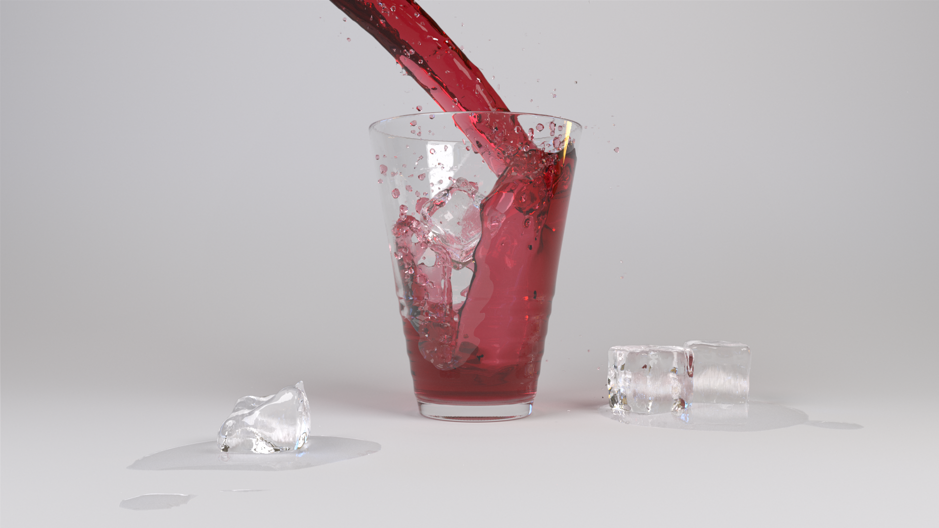
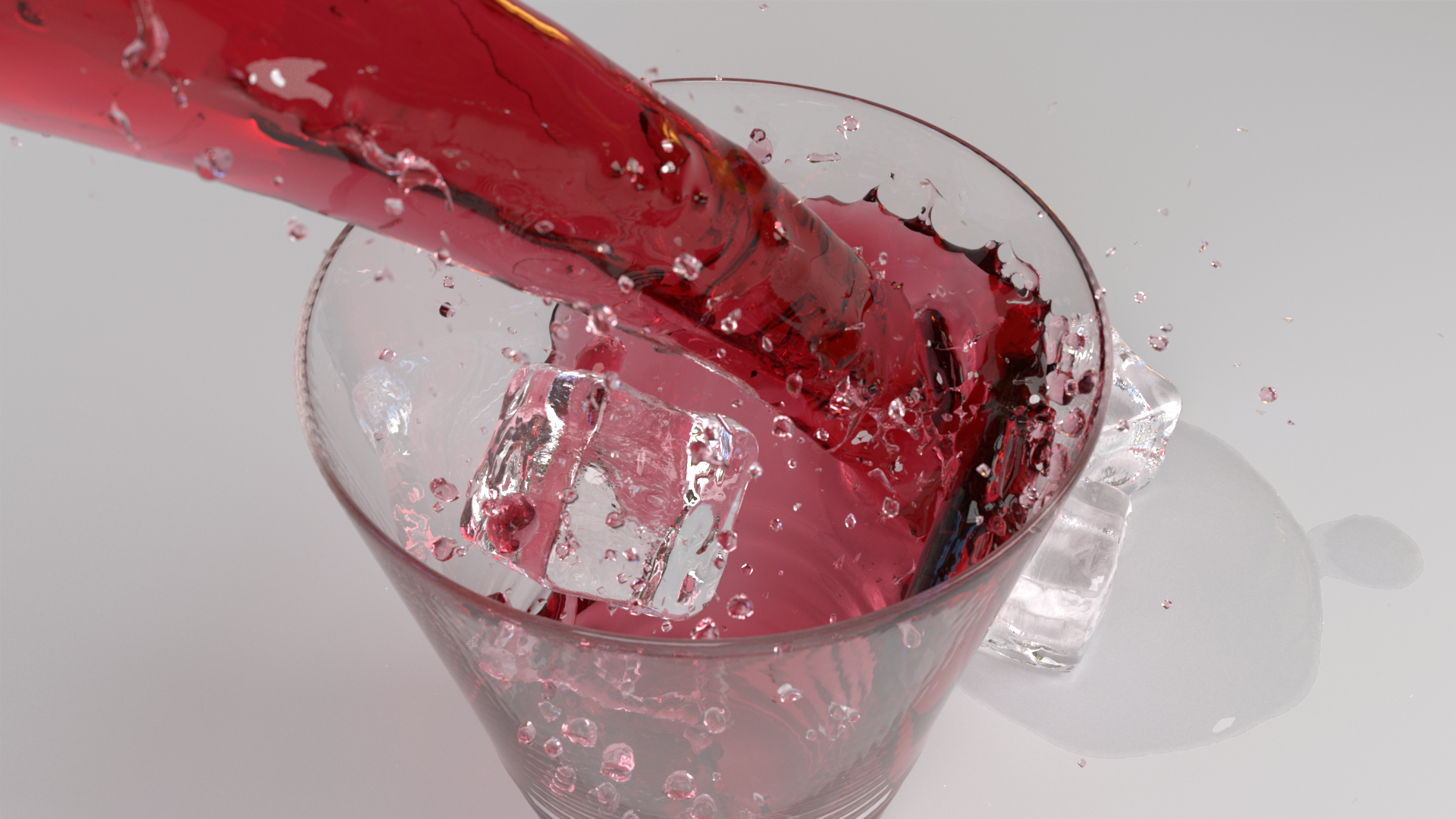
22. The Ocean and Water Pipeline of Disney’s Moana

    Sean Palmer, Jonathan Garcia, Sara Drakeley, Patrick Kelly, and Ralf Habel. The Ocean and Water Pipeline of Disney’s Moana. In ACM SIGGRAPH 2017 Talks, July 2017.

    • Preprint Version
    • Official Publisher’s Version

    Internal project from Disney Animation. This short paper describes the water pipeline developed for Moana, including the level set compositing and rendering system that was implemented in Hyperion. This system has since found additional usage on shows since Moana.

23. Recent Advancements in Disney’s Hyperion Renderer

    Brent Burley, David Adler, Matt Jen-Yuan Chiang, Ralf Habel, Patrick Kelly, Peter Kutz, Yining Karl Li, and Daniel Teece. Recent Advancements in Disney’s Hyperion Renderer. In ACM SIGGRAPH 2017 Course Notes: Path Tracing in Production Part 1, August 2017.

    • Preprint Version (Updated compared to official version)
    • Official Publisher’s Version
    • Path Tracing in Production SIGGRAPH 2017 Course

    Publication from Disney Animation. This paper describes various advancements in Hyperion since Big Hero 6 up through Moana, with a particular focus towards replacing multiple scattering approximations with true, brute-force path-traced solutions for both better artist workflows and improved visual quality.

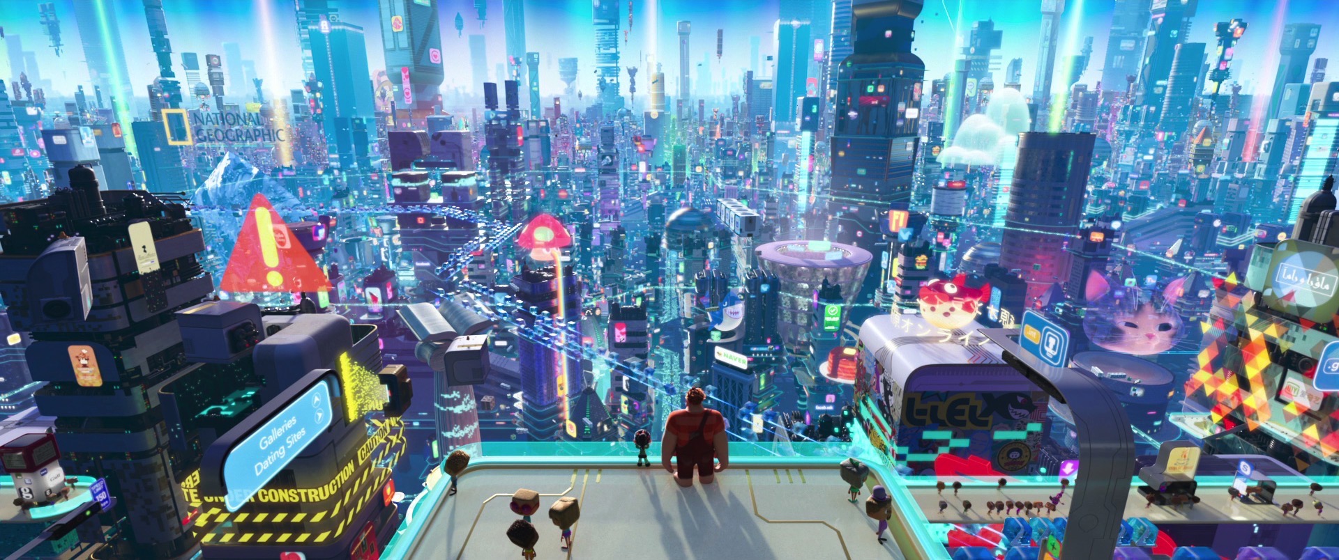
24. Denoising with Kernel Prediction and Asymmetric Loss Functions

    Thijs Vogels, Fabrice Rousselle, Brian McWilliams, Gerhard Rothlin, Alex Harvill, David Adler, Mark Meyer, and Jan Novák. Denoising with Kernel Prediction and Asymmetric Loss Functions. ACM Transactions on Graphics (Proceedings of SIGGRAPH 2018), 37(4), August 2017.

    • Preprint Version
    • Official Publisher’s Version
    • Project Page

    Joint project between DisneyResearch|Studios, Pixar, and Disney Animation. This paper describes a variety of improvements and extensions made to the 2017 Kernel-predicting Convolutional Networks for Denoising Monte Carlo Renderings paper; collectively, these improvements comprise the modern Disney-Research-developed second generation deep-learning denoiser in use in production at Pixar, ILM, and Disney Animation. At Disney Animation, used experimentally on Ralph Breaks the Internet and in full production beginning with Frozen 2.

25. Plausible Iris Caustics and Limbal Arc Rendering

    Matt Jen-Yuan Chiang and Brent Burley. Plausible Iris Caustics and Limbal Arc Rendering. ACM SIGGRAPH 2018 Talks, August 2018.

    • Preprint Version
    • Official Publisher’s Version

    Internal project from Disney Animation. This paper describes a technique for rendering realistic, physically based eye caustics using manifold next-event estimation combined with a plausible procedural geometric eye model. This realistic eye model is implemented in Hyperion and used on all projects beginning with Encanto.

26. The Design and Evolution of Disney’s Hyperion Renderer

    Brent Burley, David Adler, Matt Jen-Yuan Chiang, Hank Driskill, Ralf Habel, Patrick Kelly, Peter Kutz, Yining Karl Li, and Daniel Teece. The Design and Evolution of Disney’s Hyperion Renderer. ACM Transactions on Graphics, 37(3), August 2018.

    • Preprint Version
    • Official Publisher’s Version
    • Project Page

    Publication from Disney Animation. This paper is a systems architecture paper for the entirety of Hyperion. The paper describes the history of Disney’s Hyperion Renderer, the internal architecture, various systems such as shading, volumes, many-light sampling, emissive geometry, path simplification, fur rendering, photon-mapped caustics, subsurface scattering, and more. The paper also describes various challenges that had to be overcome for practical production use and artistic controllability. This paper covers everything in Hyperion beginning from Big Hero 6 up through Ralph Breaks the Internet.

27. Clouds Data Set

    Walt Disney Animation Studios. Clouds Data Set, August 2018.

    • Official Page
    • License

    Publicly released data set for rendering research, by Disney Animation. This data set was produced by our production artists as part of the development process for Hyperion’s modern third generation null-collision tracking based volume rendering system.

28. Moana Island Scene Data Set

    Walt Disney Animation Studios. Moana Island Scene Data Set, August 2018.

    • Official Page
    • License

    Publicly released data set for rendering research, by Disney Animation. This data set is an actual production scene from Moana, originally rendered using Hyperion and ported to PBRT v3 for the public release. This data set gives a sense of the typical scene complexity and rendering challenges that Hyperion handles every day in production.

29. Denoising Deep Monte Carlo Renderings

    Delio Vicini, David Adler, Jan Novák, Fabrice Rousselle, and Brent Burley. Denoising Deep Monte Carlo Renderings. Computer Graphics Forum, 38(1), February 2019.

    • Preprint Version
    • Official Publisher’s Version
    • Project Page

    Joint project between DisneyResearch|Studios and Disney Animation. This paper presents a technique for denoising deep (meaning images with multiple depth bins per pixel) renders, for use with deep-compositing workflows. This technique was developed as part of general denoising research from DisneyResearch|Studios and the Hyperion team.

30. The Challenges of Releasing the Moana Island Scene

    Rasmus Tamstorf and Heather Pritchett. The Challenges of Releasing the Moana Island Scene. In Proceedings of EGSR 2019, Industry Track, July 2019.

    • Preprint Version
    • Official Publisher’s Version

    Short paper from Disney Animation’s research department, discussing some of the challenges involved in preparing a production Hyperion scene for public release. The Hyperion team provided various support and advice to the larger studio effort to release the Moana Island Scene.

31. Practical Path Guiding in Production

    Thomas Müller. Practical Path Guiding in Production. In ACM SIGGRAPH 2019 Course Notes: Path Guiding in Production, July 2019.

    • Preprint Version
    • Official Publisher’s Version
    • Path Guiding in Production SIGGRAPH 2019 Course

    Joint project between DisneyResearch|Studios and Disney Animation. This paper presents a number of improvements and extensions made to Practical Path Guiding developed by in Hyperion by Thomas Müller and the Hyperion team. In use in production on Frozen 2.

32. Machine-Learning Denoising in Feature Film Production

    Henrik Dahlberg, David Adler, and Jeremy Newlin. Machine-Learning Denoising in Feature Film Production. In ACM SIGGRAPH 2019 Talks, July 2019.

    • Preprint Version
    • Official Publisher’s Version

    Joint publication from Pixar, Industrial Light & Magic, and Disney Animation. Describes how the modern Disney-Research-developed second generation deep-learning denoiser was deployed into production at Pixar, ILM, and Disney Animation.

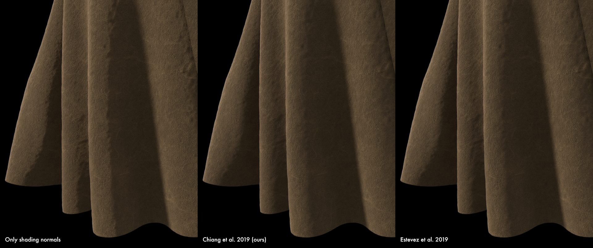
33. Taming the Shadow Terminator

    Matt Jen-Yuan Chiang, Yining Karl Li, and Brent Burley. Taming the Shadow Terminator. In ACM SIGGRAPH 2019 Talks, August 2019.

    • Preprint Version (Updated compared to official version)
    • Official Publisher’s Version
    • Project Page

    Internal project from Disney Animation. This short paper describes a solution to the long-standing “shadow terminator” problem associated with using shading normals. The technique in this paper is implemented in Hyperion and has been in use in production starting on Frozen 2 through present.

34. On Histogram-Preserving Blending for Randomized Texture Tiling

    Brent Burley. On Histogram-Preserving Blending for Randomized Texture Tiling. Journal of Computer Graphics Techniques, 8(4), November 2019.

    • Preprint Version
    • Official Publisher’s Version

    Internal project from Disney Animation. This paper describes some modiciations to the histogram-preserving hex-tiling algorithm of Heitz and Neyret; these modifications make implementing the Heitz and Neyret technique easier and more efficient. This paper describes Hyperion’s implementation of the technique, in use in production starting on Frozen 2 through present.

35. The Look and Lighting of “Show Yourself” in “Frozen 2”

    Amol Sathe, Lance Summers, Matt Jen-Yuan Chiang, and James Newland. The Look and Lighting of “Show Yourself” in “Frozen 2”. In ACM SIGGRAPH 2020 Talks, August 2020.

    • Preprint Version
    • Official Publisher’s Version

    Internal project from Disney Animation. This paper describes the process that went into achieving the final look and lighting of the “Show Yourself” sequence in Frozen 2, including a new tabulation-based approach implemented in Hyperion to maintain energy conservation in rough dielectric reflection and transmission.

36. Practical Hash-based Owen Scrambling

    Brent Burley. Practical Hash-based Owen Scrambling. Journal of Computer Graphics Techniques, 9(4), December 2020.

    • Preprint Version
    • Official Publisher’s Version

    Internal project from Disney Animation. This paper describes a new version of Owen scrambling for the Sobol sequence that is both simple to implement, efficient to evaluate, and broadly applicable to various problems.

37. Unbiased Emission and Scattering Importance Sampling For Heterogeneous Volumes

    Wei-Feng Wayne Huang, Peter Kutz, Yining Karl Li, and Matt Jen-Yuan Chiang. Unbiased Emission and Scattering Importance Sampling For Heterogeneous Volumes. In ACM SIGGRAPH 2021 Talks, August 2021.

    • Preprint Version
    • Official Publisher’s Version
    • Project Page

    Internal project from Disney Animation. This paper describes a pair of new unbiased distance-sampling methods for production volume path tracing, with a specific focus on sampling emission and scattering. First used on Raya and the Last Dragon.

38. The Atmosphere of Raya and the Last Dragon

    Marc Bryant, Ryan DeYoung, Wei-Feng Wayne Huang, Joe Longson, and Noel Villegas. The Atmosphere of Raya and the Last Dragon. In ACM SIGGRAPH 2021 Talks, August 2021.

    • Preprint Version
    • Official Publisher’s Version

    Internal project from Disney Animation. This paper describes the various rendering and workflow improvements that went into rendering atmospheric volumes to produce the highly atmospheric lighting in Raya and the Last Dragon.

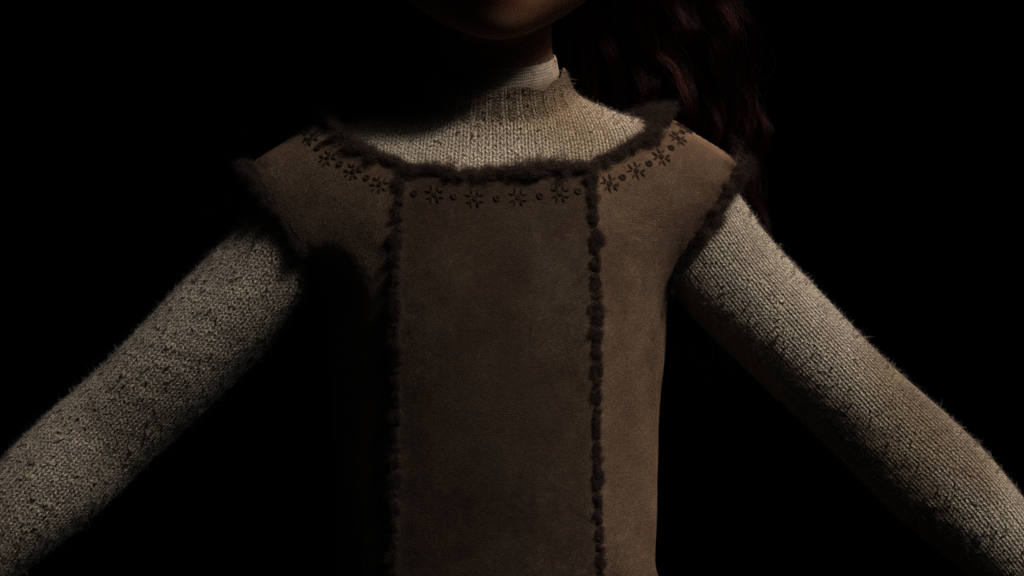
39. Practical Multiple-Scattering Sheen Using Linearly Transformed Cosines

    Tizian Zeltner, Brent Burley, and Matt Jen-Yuan Chiang. Practical Multiple-Scattering Sheen Using Linearly Transformed Cosines. In ACM SIGGRAPH 2022 Talks, August 2022.

    • Preprint Version
    • Official Publisher’s Version
    • Project Page

    Joint project between École Polytechnique Fédérale de Lausanne (EPFL) and Disney Animation. This paper descibes the new multiple-scattering sheen model used in the Disney Principled BSDF starting with the production of Strange World.

40. Deep Adaptive Sampling and Reconstruction Using Analytic Distributions

    Farnood Salehi, Marco Manzi, Gerhard Rothlin, Romann Weber, Christopher Schroers, and Marios Papas. Deep Adaptive Sampling and Reconstruction Using Analytic Distributions. ACM Transactions on Graphics (Proceedings of SIGGRAPH Asia 2022), 41(6), December 2022.

    • Preprint Version
    • Official Publisher’s Version
    • Project Page

    External project from DisneyResearch|Studios, with project support from Disney Animation. This paper extends Disney’s deep learning denoising technology to also drive adaptive sampling during the rendering process. Part of a larger joint research project between DisneyResearch|Studios, Disney Animation, Pixar, and Industrial Light & Magic on denoising techniques.

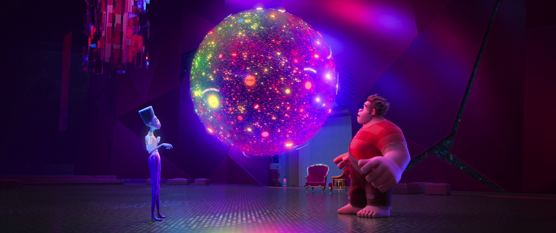
41. “Encanto” - Let’s Talk About Bruno’s Visions

    Corey Butler, Brent Burley, Wei-Feng Wayne Huang, Yining Karl Li, and Benjamin Huang. “Encanto” - Let’s Talk About Bruno’s Visions. In ACM SIGGRAPH 2022 Talks, August 2022.

    • Preprint Version
    • Official Publisher’s Version
    • Project Page

    Internal project from Disney Animation. This paper describes the process of creating the holographic prophecy shards from Encanto, including a new teleportation shader in Hyperion that was developed specifically to support this effect.

42. Fracture-Aware Tessellation of Subdivision Surfaces

    Brent Burley and Francisco Rodriguez. Fracture-Aware Tessellation of Subdivision Surfaces. In ACM SIGGRAPH 2022 Talks, August 2022.

    • Preprint Version
    • Official Publisher’s Version

    Internal project from Disney Animation. This paper describes a new tessellation algorithm for fractured subdivision surfaces, used as part of Disney Animation’s destruction FX pipeline and implemented in Hypeprion. First used in production on Encanto.

43. Deep Compositional Denoising on Frame Sequences

    Xianyao Zhang, Gerhard Rothlin, Marco Manzi, Markus Gross, and Marios Papas. Deep Compositional Denoising on Frame Sequences. In EGSR 2023: Proceedings of the 34th Eurographics Symposium on Rendering, June 2023.

    • Preprint Version
    • Official Publisher’s Version
    • Project Page

    External project from DisneyResearch|Studios, with project support from Disney Animation. This paper unifies previously separate approaches used in Disney’s deep learning denoising system for single-frame compositional denoising and multi-frame non-compositional denoising. Part of a larger joint research project between DisneyResearch|Studios, Disney Animation, Pixar, and Industrial Light & Magic on denoising techniques.

44. Progressive Null-Tracking for Volumetric Rendering

    Zackary Misso, Yining Karl Li, Brent Burley, Daniel Teece, and Wojciech Jarosz. Progressive Null Tracking for Volumetric Rendering. SIGGRAPH ‘23: ACM SIGGRAPH 2023 Conference Proceedings, August 2023.

    • Preprint Version
    • Official Publisher’s Version
    • Project Page

    Joint project between Dartmouth College and Disney Animation. This paper describes a new method to progressively learn bounding majorants when using null-tracking techniques to perform unbiased rendering of general heterogeneous volumes with unknown bounding majorants.

45. Splat: Developing a ‘Strange’ Shader

    Kendall Litaker, Brent Burley, Dan Lipson, and Mason Khoo. Splat: Developing a ‘Strange’ Shader. In ACM SIGGRAPH 2023 Talks, August 2023.

    • Preprint Version
    • Official Publisher’s Version

    Internal project from Disney Animation. This paper describes the unusual challenges encountered when developing the unique shading and look for the Splat character from Strange World.

46. Neural Denoising for Deep-Z Monte Carlo Renderings

    Xianyao Zhang, Gerhard Rothlin, Shilin Zhu, Tunç Ozan Aydin, Farnood Salehi, Markus Gross, Marios Papas. Neural Denoising for Deep-Z Monte Carlo Renderings. Computer Graphics Forum (Proceedings of Eurographics 2024), 43(2), April 2024.

    • Preprint Version
    • Official Publisher’s Version
    • Project Page

    External joint project between DisneyResearch|Studios and Pixar, with project support from Disney Animation. This paper describes an extension to Disney’s deep learning denoising technology to add support for deep-Z images and deep compositing workflows. Part of a larger joint research project between DisneyResearch|Studios, Disney Animation, Pixar, and Industrial Light & Magic on denoising techniques.

47. Cache Points for Production-Scale Occlusion-Aware Many-Lights Sampling and Volumetric Scattering

    Yining Karl Li, Charlotte Zhu, Gregory Nichols, Peter Kutz, Wei-Feng Wayne Huang, David Adler, Brent Burley, and Daniel Teece. Cache Points for Production-Scale Occlusion-Aware Many-Lights Sampling and Volumetric Scattering. In DigiPro ‘24: Proceedings of the Digital Production Symposium 2024, July 2024.

    • Preprint Version
    • Official Publisher’s Version
    • Project Page

    Internal project from Disney Animation. This paper describes Hyperion’s unique many-lights importance sampling system. Used on every project rendered using Hyperion to date, this paper contains deep implementation details and notes from a decade of production experience.

48. Dynamic Screen Space Textures for Coherent Stylization

    Brent Burley, Brian Green, and Daniel Teece. Dynamic Screen Space Textures for Coherent Stylization. In ACM SIGGRAPH 2024 Talks, July 2024.

    • Preprint Version
    • Official Publisher’s Version

    Internal project from Disney Animation. This paper describes a novel new dynamic screen space texturing system that makes up a key part of the stylized watercolor look of Wish.

49. Volume Scattering Probability Guiding

    Kehan Xu, Sebastian Herholz, Marco Manzi, Marios Papas, and Markus Gross. Volume Scattering Probability Guiding. ACM Transactions on Graphics (Proceedings of SIGGRAPH Asia 2024), 43(6), December 2024.

    • Preprint Version
    • Official Publisher’s Version
    • Project Page

    External joint project between DisneyResearch|Studios and Intel, with project support from Disney Animation. This paper describes an improvement to volume path guiding that enables direct control over volume scattering probability. Part of a larger joint research project between DisneyResearch|Studios, Disney Animation, Pixar, and Industrial Light & Magic on path guiding techniques.

50. Neural Resampling with Optimized Candidate Allocation

    Alexander Rath, Marco Manzi, Farnood Salehi, Sebastian Weiss, Tiziano Portenier, Saeed Hadadan, and Marios Papas. Neural Resampling with Optimized Candidate Allocation. In EGSR 2025: Proceedings of the 36th Eurographics Symposium on Rendering, June 2025.

    • Preprint Version
    • Official Publisher’s Version

    Joint project between DisneyResearch|Studios and Disney Animation. This paper presents an experimental implementation of GPU-based neural learning system inside of Hyperion’s CPU-based architecture, suitable for use as both a path guiding system and for radiance caching. Part of a larger joint research project between DisneyResearch|Studios, Disney Animation, Pixar, and Industrial Light & Magic on path guiding techniques.

51. A Texture Streaming Pipeline for Real-Time GPU Ray Tracing

    Mark Lee, Nathan Zeichner, and Yining Karl Li. A Texture Streaming Pipeline for Real-Time GPU Ray. In ACM SIGGRAPH 2025 Talks, August 2025.

    • Preprint Version
    • Official Publisher’s Version
    • Project Page

    Internal project from Disney Animation. This paper describes our implementation of a streaming textures system on the GPU for Ptex, which is in use in our in-house GPU path tracing previsualization renderer.

52. Path Guiding Surfaces and Volumes in Disney’s Hyperion Renderer: A Case Study

    Lea Reichardt, Brian Green, Yining Karl Li, and Marco Manzi. Path Guiding Surfaces and Volumes in Disney’s Hyperion Renderer: A Case Study. In ACM SIGGRAPH 2025 Course Notes: Path Guiding in Production and Recent Advancements, August 2025.

    • Preprint Version (Hyperion Chapter)
    • Preprint Version (Full Course Notes)
    • Official Publisher’s Version
    • Path Guiding in Production and Recent Advancements SIGGRAPH 2025 Course

    Joint project from DisneyResearch|Studios and Disney Animation. This paper describes how we’ve implemented Hyperion’s second-generation path guiding system, and what we’ve learned from bridging cutting edge research into production usage.

Additional Resources

Again, this post is meant to be a living document; any new publications with involvement from the Hyperion team will be added here. Of course, the Hyperion team is not the only team at Disney Animation that regularly publishes; for a full list of publications from Disney Animation, see the official Disney Animation publications page. The Disney Animation Technology website is also worth keeping an eye on if you want to keep up on what our engineers and TDs are working on!

If you’re just getting started and want to learn more about rendering in general, the must-read text that every rendering engineer has on their desk or bookshelf is Physically Based Rendering 3rd Edition by Matt Pharr, Wenzel Jakob, and Greg Humphreys (now available online completely for free!). Also, the de-facto standard beginner’s text today is the Ray Tracing in One Weekend series by Peter Shirley, which provides a great, gentle, practical introduction to ray tracing, and is also available completely for free. Also take a look at Real-Time Rendering 4th Edition, Ray Tracing Gems (also available online for free), The Graphics Codex by Morgan McGuire, and Eric Haines’s Ray Tracing Resources page.

Many other amazing rendering teams at both large studios and commercial vendors also publish regularly, and I highly recommend keeping up with all of their work too! For a good starting point into exploring the wider world of production rendering, check out the ACM Transactions on Graphics Special Issue on Production Rendering, which is edited by Matt Pharr and contains extensive, detailed systems papers on Pixar’s RenderMan, Weta Digital’s Manuka, Solid Angle (Autodesk)’s Arnold, Sony Picture Imageworks’ Arnold, and of course Disney Animation’s Hyperion. A sixth paper that I would group with five above is the High Performance Graphics 2017 paper detailing the architecture of DreamWorks Animation’s MoonRay.

For even further exploration, extensive course notes are available from SIGGRAPH courses every year. Particularly good recurring courses to look at from past years are the Path Tracing in Production course (2017, 2018, 2019), the absolutely legendary Physically Based Shading course (2010, 2012, 2013, 2014, 2015, 2016, 2017), the various incarnations of a volume rendering course (2011, 2017, 2018), and now due to the dawn of ray tracing in games, Advances in Real-Time Rendering and Open Problems in Real-Time Rendering. Also, Stephen Hill typically collects links to all publicly available course notes, slides, source code, and more for SIGGRAPH each year after the conference on his blog; both his blog and the blogs listed on the sidebar of his website are essentially mandatory reading in the rendering world. Also, interesting rendering papers are always being published in journals and at conferences. The major journals to check are ACM Transactions on Graphics (TOG), Computer Graphics Forum (CGF), and the Journal of Computer Graphics Techniques (JCGT); the major academic conferences where rendering stuff appears are SIGGRAPH, SIGGRAPH Asia, EGSR (Eurographics Symposium on Rendering), HPG (High Performance Graphics), MAM (Workshop on Material Appearance Modeling), EUROGRAPHICS, and i3D (ACM SIGGRAPH Symposium on Interactive 3D Graphics and Games); another three industry conferences where interesting stuff often appears are DigiPro, GDC (Game Developers Conference) and GTC (Graphics Technology Conference). A complete listing of the contents for all of these conferences every year, along with links to preprints, is compiled by Ke-Sen Huang.

Contributors

A large number of people have contributed directly to Hyperion’s development since the beginning of the project, in a variety of capacities ranging from core developers to TDs and support staff and all the way to notable interns. In no particular order, including both present and past: Daniel Teece, Brent Burley, David Adler, Yining Karl Li, Mark Lee, Charlotte Zhu, Brian Green, Andrew Bauer, Lea Reichardt, Mackenzie Thompson, Wei-Feng Wayne Huang, Matt Jen-Yuan Chen, Joe Schutte, Andrew Gartner, Jennifer Yu, Peter Kutz, Ralf Habel, Patrick Kelly, Gregory Nichols, Andrew Selle, Christian Eisenacher, Jan Novák, Ben Spencer, Doug Lesan, Lisa Young, Tami Valdez, Andrew Fisher, Noah Kagan, Benedikt Bitterli, Thomas Müller, Tizian Zeltner, Zackary Misso, Magdalena Martinek, Mathijs Molenaar, Laura Lediav, Guillaume Loubet, David Koerner, Simon Kallweit, Gabor Liktor, Ulrich Muller, Norman Moses Joseph, Stella Cheng, Marc Cooper, Tal Lancaster, and Serge Sretschinsky. Over the years, our closest research partners at DisneyResearch|Studios, Pixar Animation Studios, Industrial Light & Magic, and elsewhere have included (in no particular order): Marios Papas, Marco Manzi, Tiziano Portenier, Alexander Rath, Rajesh Sharma, Rasmus Tamstorf, Jan Novák, Gerhard Roethlin, Per Christensen, Julian Fong, Mark Meyer, André Mazzone, Wojciech Jarosz, Fabrice Rouselle, Christophe Hery, Ryusuke Villemin, and Magnus Wrenninge. Invaluable support from studio leadership over the years has been provided by (again, in no particular order): Nick Cannon, Munira Tayabji, Rebecca Bever, Bettina Martin, Laura Franek, Collin Larkins, Golriz Fanai, Rajesh Sharma, Chuck Tappan, Sean Jenkins, Darren Robinson, Alex Nijmeh, Hank Driskill, Kyle Odermatt, Adolph Lusinsky, Ernie Petti, Kelsey Hurley, Shweta Viswanathan, Tad Miller, Mark Hammel, Mohit Kallianpur, Brian Leach, Daniel Rice, Amol Sathe, Alessandro Jacomini, Josh Staub, Steve Goldberg, Scott Kersavage, Andy Hendrickson, Dan Candela, Ed Catmull, and many others. Of course, beyond this enormous list, there is an even more enormous list of countless artists, technical directors, production supervisors, and other technology development teams at Disney Animation who motivated Hyperion, participated in its development, and contributed to its success. If anything in this post has caught your interest, keep an eye out for open position listings on DisneyAnimation.com; maybe these lists can one day include you!

Made with Hyperion

Finally, here is a list of all publicly released and announced projects to date made using Disney’s Hyperion Renderer:

Feature Films: Big Hero 6 (2014), Zootopia (2016), Moana (2016), Ralph Breaks the Internet (2018), Frozen 2 (2019), Raya and the Last Dragon (2021), Encanto (2021), Strange World (2022), Wish (2023), Moana 2 (2024), Zootopia 2 (2025)

Shorts and Featurettes: Feast (2014), Frozen Fever (2015), Inner Workings (2016), Gone Fishing (2017), Olaf’s Frozen Adventure (2017), Myth: A Frozen Tale¹ (2019), Once Upon a Snowman (2020), Us Again (2021), Far from the Tree (2021), Once Upon a Studio (2023), Versa (2025)

Animated Series: At Home With Olaf (2020), Olaf Presents (2021), Baymax! (2022), Zootopia+ (2022)

Short Circuit Shorts: Exchange Student (2020), Just a Thought (2020), Jing Hua (2020), Elephant in the Room (2020), Puddles (2020), Lightning in a Bottle (2020), Zenith (2020), Drop (2020), Fetch (2020), Downtown (2020), Hair-Jitsu (2020), The Race (2020), Lucky Toupée (2020), Cycles² (2020), A Kite’s Tale² (2020), Going Home (2021), Crosswalk (2021), Songs to Sing in the Dark (2021), No. 2 to Kettering (2021), Reflect (2022), Life Drawings (2026), Maddie & the Test (2026)

Intern Shorts: Ventana (2017), Voilà (2018), Maestro (2019), June Bug (2021)

Filmmaker Co-op Shorts: Weeds (2017), Forevergreen (2025)

Disney Parks Rides³: Zootopia: Hot Pursuit (Shanghai Disneyland, 2023), Peter Pan’s Never Land Adventure (Tokyo DisneySea, 2024), Zootopia: Better Zoogether! (Disney’s Animal Kingdom, 2025)

Footnotes

¹ VR project running on Unreal Engine, with shading and textures baked out of Disney’s Hyperion Renderer. keyboard_return

² VR project running on Unity, with shading and textures baked out of Disney’s Hyperion Renderer. keyboard_return

³ CG animation provided by Disney Animation, incorporated into park rides built by Walt Disney Imagineering. keyboard_return

Table of Contents

Introduction

A few years ago, I wrote a post about attenuated transmission and what I called “deep attenuation” at the time- refraction and transmission through multiple mediums embedded inside of each other, a.k.a. what is usually called nested dielectrics. What I called “deep attenuation” in that post is, in its essence, just pure interface tracking using a stack. This post is meant as a revisit and update of that post; I’ll talk about the problems with the ad-hoc pure interface tracking technique I came up with in that previous post and discuss the proper priority-based nested dielectric technique [Schmidt and Budge 2002] that Takua uses today.

In my 2015 post, I included a diagram showing the overlapping boundaries required to model ice cubes in a drink in a glass, but I didn’t actually include a render of that scenario! In retrospect, the problems with the 2015 post would have become obvious to me more quickly if I had actually done a render like that diagram. Figure 1 shows an actual “ice cubes in a drink in a glass” scene, rendered correctly using Takua Renderer’s implementation of priority-based nested dielectrics. For comparison, Figure 2 shows what Takua produces using the approach in the 2015 post; there are a number of obvious bizarre problems! In Figure 2, the ice cubes don’t properly refract the tea behind and underneath them, and the ice cubes under the liquid surface aren’t visible at all. Also, where the surface of the tea interfaces with the glass teacup, there is a odd bright ring. Conversely, Figure 1 shows a correct liquid-glass interface without a bright ring, shows proper refraction through the ice cubes, and correctly shows the ice cubes under the liquid surface.

Problems with only Interface Tracking

So what exactly is wrong with using only interface tracking without priorities? First, let’s quickly summarize how my old interface tracking implementation worked. Note that here we refer to the side of a surface a ray is currently on as the incident side, and the other side of the surface as the transmit side. For each path, keep a stack of which Bsdfs the path has encountered:

• When a ray enters a surface, push the encountered surface onto the stack.
• When a ray exits a surface, scan the stack from the top down and pop the first instance of a surface in the stack matching the encountered surface.
• When hitting the front side of a surface, the incident properties comes from the top of the stack (or is the empty default if the stack is empty), and the transmit properties comes from surface being intersected.
• When hitting the back side of a surface, the incident properties comes from the surface being intersected, and the transmit properties comes from the top of the stack (or is the empty default if the stack is empty).
• Only push/pop onto the stack when a refraction/transmission event occurs.

Next, as an example, imagine a case where which surface a ray currently in is ambiguous. A common example of this case is when two surfaces are modeled as being slightly overlapping, as is often done when modeling liquid inside of a glass since modeling perfectly coincident surfaces in CG is either extremely difficult or impossible due to floating point precision problems. Even if we could model perfectly coincident surfaces, rendering perfectly coincident surfaces without artifacts is similarly extremely difficult or impossible, also due to floating point precision problems. Figure 3 shows a diagram of how a glass containing water and ice cubes is commonly modeled; in Figure 3, the ambiguous regions are where the water surface is inside of the glass and inside of the ice cube. When a ray enters this overlapping region, it is not clear whether we should treat the ray as being inside the water or inside if the glass (or ice)!

Using the pure interface tracking algorithm from my old blog post, below is what happens at each path vertex along the path illustrated in Figure 3. In this example, we define the empty default to be air.

1. Enter Glass.
   • Incident/transmit IOR: Air/Glass.
   • Push Glass onto stack. Stack after event: (Glass).
2. Enter Water.
   • Incident/transmit IOR: Glass/Water.
   • Push Water onto stack. Stack after event: (Water, Glass).
3. Exit Glass.
   • Incident/transmit IOR: Glass/Water.
   • Remove Glass from stack. Stack: (Water).
4. Enter Ice.
   • Incident/transmit IOR: Water/Ice.
   • Push Ice onto stack. Stack: (Ice, Water).
5. Exit Water.
   • Incident/transmit IOR: Water/Ice.
   • Remove Water from stack. Stack: (Ice).
6. Exit Ice.
   • Incident/transmit IOR: Ice/Air.
   • Remove Ice from stack. Stack: empty.
7. Enter Water.
   • Incident/transmit IOR: Air/Water.
   • Push Water onto stack. Stack after event: (Water).
8. Enter Glass.
   • Incident/transmit IOR: Water/Glass.
   • Push Glass onto stack. Stack after event: (Glass, Water).
9. Reflect off Water.
   • Incident/transmit IOR: Water/Glass.
   • No change to stack. Stack after event: (Glass, Water).
10. Reflect off Glass.
    • Incident/transmit IOR: Glass/Glass.
    • No change to stack. Stack after event: (Glass, Water).
11. Exit Water.
    • Incident/transmit IOR: Water/Glass.
    • Remove Water from stack. Stack after event: (Glass).
12. Exit Glass.
    • Incident/transmit IOR: Glass/Air.
    • Remove Glass from stack. Stack after event: empty.

Observe events 3 and 5, where the same index of refraction boundary is encountered as in the previous event. These double events are where some of the weirdness in Figure 2 comes from; specifically the bright ring at the liquid-glass surface interface and the incorrect refraction through the ice cube. These double events are not actually physically meaningful; in reality, a ray could never be both inside of a glass surface and inside of a water surface simultaneously. Figure 4 shows a simplified version of the tea cup example above, without ice cubes; even then, the double event still causes a bright ring at the liquid-glass surface interface. Also note how when following the rules from my old blog post, event 10 becomes a nonsense event where the incident and transmit IOR are the same. The fix for this case is to modify the rules so that when a ray exits a surface, the transmit properties come from the first surface on the stack that isn’t the same as the incident surface, but even with this fix, the reflection at event 10 is still physically impossible.

Really what we want is to model overlapping surfaces, but then in overlapping areas, be able to specify which surface a ray should think it is actually inside of. Essentially, this functionality would make overlapping surfaces behave like boolean operators; we would be able to specify that the ice cubes in Figure 3 “cut out” a space from the water they overlap with, and the glass cut out a space from the water as well. This way, the double events never occur since rays wouldn’t see the second event in each pair of double events. One solution that immediately comes to mind is to simply consider whatever surface is at the top of the interface tracking stack as being the surface we are currently inside, but this causes an even worse problem: the order of surfaces that a ray thinks it is in becomes dependent on what surfaces a ray encounters first, which depends on the direction and location of each ray! This produces an inconsistent view of the world across different rays. Instead, a better solution is provided by priority-based nested dielectrics [Schmidt and Budge 2002].

Priority-Based Nested Dielectrics

Priority-based nested dielectrics work by assigning priority values to geometry, with the priority values determining which piece of geometry “wins” when a ray is in a region of space where multiple pieces of geometry overlap. A priority value is just a single number assigned as an attribute to a piece of geometry or to a shader; the convention established by the paper is that lower numbers indicate higher priority. The basic algorithm in [Schmidt and Budge 2002] works using an interior list, which is conceptually similar to an interface tracking stack. The interior list is exactly what it sounds like: a list of all of the surfaces that a path has entered but not exited yet. Unlike the interface tracking stack though, the interior list doesn’t necessarily have to be a stack or have any particular ordering, although implementing it as a list always sorted by priority may provide some minor practical advantages. When a ray hits a surface during traversal, the following rules apply:

• If the surface has a higher or equal priority (so lower or equal priority number) than anything else on the interior list, the result is a true hit and a intersection has occured. Proceed with regular shading and Bsdf evaluation.
• If the surface has a lower priority (so higher priority number) than the highest-priority value on the interior list, the result is a false hit and no intersection has occured. Ignore the intersection and continue with ray traversal.
• If the hit is a false hit OR if the hit both is a true hit and results in a refraction/transmission event:
  • Add the surface to the interior list if the ray is entering the surface.
  • Remove the surface from the interior list if the ray is exiting the surface.
• For a true hit the produces a reflection event, don’t add the surface to the interior list.

Note that this approach only works with surfaces that are enclosed manifolds; that is, every surface defines a finite volume. When a ray exits a surface, the surface it is exiting must already be in the interior list; if not, then the interior list can become corrupted and the renderer may start thinking that paths are in surfaces that they are not actually in (or vice verse). Also note that a ray can only ever enter into a higher-priority surface through finding a true hit, and can only enter into a lower-priority surface by exiting a higher-priority surface and removing the higher-priority surface from the interior list. At each true hit, we can figure out the properties of the incident and transmit sides by examining the interior list. If hitting the front side of a surface, before we update the interior list, the surface we just hit provides the transmit properties and the highest-priority surface on the interior list provides the incident properties. If hitting the back side of a surface, before we update the interior list, the surface we just hit provides the incident properties and the second-highest-priority surface on the interior list provides the transmit properties. Alternatively, if the interior list only contains one surface, then the transmit properties come from the empty default. Importantly, if a ray hits a surface with no priority value set, that surface should always count as a true hit. This way, we can embed non-transmissive objects inside of transmissive objects and have everything work automatically.

Figure 5 shows the same scenario as in Figure 3, but now with priority values assigned to each piece of geometry. The path depicted in Figure 5 uses the priority-based interior list; dotted lines indicate parts of a surface that produce false hits due to being embedded within a higher-priority surface:

The empty default air surrounding everything is defined as having an infinitely high priority value, which means a lower priority than any surface in the scene. Using the priority-based interior list, here are the events that occur at each intersection along the path in Figure 5:

1. Enter Glass.
   • Glass priority (1) is higher than ambient air (infinite), so TRUE hit.
   • Incident/transmit IOR: Air/Glass.
   • True hit, so evaluate Bsdf and produce refraction event.
   • Interior list after event: (Glass:1). Inside surface after event: Glass.
2. Enter Water.
   • Water priority (2) is lower than highest priority in interior list (1), so FALSE hit.
   • Incident/transmit IOR: N/A.
   • False hit, so do not evaluate Bsdf and just continue straight.
   • Interior list after event: (Glass:1, Water:2). Inside surface after event: Glass.
3. Exit Glass.
   • Glass priority (1) is equal to the highest priority in interior list (1), so TRUE hit.
   • Incident/transmit IOR: Glass/Water.
   • True hit, so evaluate Bsdf and produce refraction event. Remove Glass from interior list.
   • Interior list after event: (Water:2). Inside surface after event: Water.
4. Enter Ice.
   • Ice priority (0) is higher than the highest priority in interior list (2), so TRUE hit.
   • Incident/transmit IOR: Water/Ice.
   • True hit, so evaluate Bsdf and produce refraction event.
   • Interior list after event: (Water:2, Ice:0). Inside surface after event: Ice.
5. Exit Water.
   • Ice priority (0) is higher than the highest priority in interior list (2), so TRUE hit.
   • Incident/transmit IOR: N/A.
   • False hit, so do not evaluate Bsdf and just continue straight. Remove Water from interior list.
   • Interior list after event: (Ice:0). Inside surface after event: Ice.
6. Exit Ice.
   • Ice priority is only surface in the interior list, so TRUE hit.
   • Incident/transmit IOR: Ice/Air.
   • True hit, so evaluate Bsdf and produce refraction event. Remove Ice from interior list.
   • Interior list after event: empty. Inside surface after event: air.
7. Enter Water.
   • Water priority (2) is higher than ambient air (infinite), so TRUE hit.
   • Incident/transmit IOR: Air/Water.
   • True hit, so evaluate Bsdf and produce refraction event.
   • Interior list after event: (Water:2). Inside surface after event: Water.
8. Enter Glass.
   • Glass priority (1) is higher than the highest priority in interior list (2), so TRUE hit.
   • Incident/transmit IOR: Water/Glass.
   • True hit, so evaluate Bsdf and produce refraction event.
   • Interior list after event: (Water:2, Glass:1). Inside surface after event: Glass.
9. Exit Water.
   • Water priority (2) is lower than highest priority in interior list (1), so FALSE hit.
   • Incident/transmit IOR: N/A.
   • False hit, so do not evaluate Bsdf and just continue straight.
   • Interior list after event: (Glass:1). Inside surface after event: Glass.
10. Reflect off Glass.
    • Glass priority (1) is equal to the highest priority in interior list (1), so TRUE hit.
    • Incident/transmit IOR: Glass/Air.
    • True hit, so evaluate Bsdf and produce reflection event.
    • Interior list after event: (Glass:1). Inside surface after event: Glass.
11. Enter Water.
    • Water priority (2) is lower than highest priority in interior list (1), so FALSE hit.
    • Incident/transmit IOR: N/A.
    • False hit, so do not evaluate Bsdf and just continue straight.
    • Interior list after event: (Glass:1, Water:2). Inside surface after event: Glass.
12. Reflect off Glass.
    • Glass priority (1) is equal to the highest priority in interior list (1), so TRUE hit.
    • Incident/transmit IOR: Glass/Water.
    • True hit, so evaluate Bsdf and produce reflection event.
    • Interior list after event: (Glass:1, Water:2). Inside surface after event: Glass.
13. Exit Water.
    • Water priority (2) is lower than highest priority in interior list (1), so FALSE hit.
    • Incident/transmit IOR: N/A.
    • False hit, so do not evaluate Bsdf and just continue straight.
    • Interior list after event: (Glass:1). Inside surface after event: Glass.
14. Exit Glass.
    • Glass priority (1) is equal to the highest priority in interior list (1), so TRUE hit.
    • Incident/transmit IOR: Glass/Air.
    • True hit, so evaluate Bsdf and produce refraction event. Remove Glass from interior list.
    • Interior list after event: empty. Inside surface after event: air.

The entire above sequence of events is physically plausible, and produces no weird double-events! Using priority-based nested dielectrics, Takua generates the correct images in Figure 1 and Figure 6. Note how in Figure 6 below, the liquid appears to come right up against the glass, without any bright boundary artifacts or anything else.

For actually implementing priorty-based nested dielectrics in a ray tracing renderer, I think there are two equally plausible places in the renderer where the implementation can take place. The first and most obvious location is as part of standard light transport integration or shading system. The integrator would be in charge of checking for false hits and tracing continuation rays through false hit geometry. A second, slightly less obvious location is actually as part of ray traversal through the scene itself. Including handling of false hits in the traversal system can be more efficient than handling it in the integrator since the false hit checks could be done in the middle of a single BVH tree traversal, whereas handling false hits by firing continuation rays requires a new BVH tree traversal for each false hit encountered. Also, handling false hits in the traversal system removes some complexity from the integrator. However, the downside to handling false hits in the traversal system is that it requires plumbing all of the interior list data and logic into the traversal system, which sets up something of a weird backwards dependency between the traversal and shading/integration systems. I wound up choosing to implement priority-based nested dielectrics in the integration system in Takua, simply to avoid having to do complex, weird plumbing back into the traversal system. Takua uses priority-based nested dielectrics in all integrators, including unidirectional path tracing, BDPT, PPM, and VCM, and also uses the nested dielectrics system to handle transmittance along bidirectional connections through attenuating mediums.

Even though the technique has “nested dielectrics” in the title, this technique is not in principle limited to only dielectrics. In Takua, I now use this technique to handle all transmissive cases, including for both dielectric surfaces and for surfaces with diffuse transmission. Also, in addition to just determining the incident and transmit IORs, Takua uses this system to also determine things like what kind of participating medium a ray is currently inside of in order to calculate attenuation. This technique appears to be more or less the industry standard today; implementations are available for at least Renderman, Arnold, Mantra, and Maxwell Render.

As a side note, during the course of this work, I also upgraded Takua’s attenuation system to use ratio tracking [Novák et al. 2014] instead of ray marching when doing volumetric lookups. This change results in an important improvement to the attenuation system: ratio tracking provides an unbiased estimate of transmittance, whereas ray marching is inherently biased due to being a quadrature-based technique.

Figures 7 and 8 show a fancier scene of liquid pouring into a glass with some ice cubes and such. This scene is the Glass of Water scene from Benedikt Bitterli’s rendering resources page [Bitterli 2016], modified with brighter lighting on a white backdrop and with red liquid. I also had to modify the scene so that the liquid overlaps the glass slightly; providing a clearer read for the liquid-glass interface is why I made the liquid red. One of the neat features of this scene are the cracks modeled inside of the ice cubes; the cracks are non-manifold geometry. To render them correctly, I applied a shader with glossy refraction to the crack geometry but did not set a priority value for them; this works correctly because the cracks, being non-manifold, don’t have a concept of inside or outside anyway, so they should not participate in any interior list considerations.

References

Benedikt Bitterli. 2016. Rendering Resources. Retrieved from https://benedikt-bitterli.me/resources/.

Jan Novák, Andrew Selle and Wojciech Jarosz. 2014. Residual Ratio Tracking for Estimating Attenuation in Participating Media. ACM Transactions on Graphics (Proc. of SIGGRAPH Asia) 33, 6 (Nov. 2014), Article 179.

Charles M. Schmidt and Brian Budge. 2002. Simple Nested Dielectrics in Ray Traced Images. Journal of Graphics Tools 7, 2 (Jan. 2002), 1–8.

Some Blog Update Notes

For the past few years, my blog posts covering personal work have trended towards gignormous epic articles tackling huge subjects published only once or twice a year, such as with the bidirectional mipmapping post and its promised but still unfinished part 2. Unfortunately, I’m not the fastest writer when working on huge posts, since writing those posts often involves significant learning and multiple iterations of implementation and testing on my part. Over the next few months, I’m aiming to write more posts similar to this one, covering some relatively smaller topics, so that I can get posts coming out a bit more frequently while I continue to work on several upcoming, gignormous posts on long-promised topics. Or at least, that’s the plan… we’ll see!

The Walt Disney Animation Studios film for 2018 is Ralph Breaks the Internet, which is the sequel to 2012’s Wreck-It Ralph. Over the past two years, I’ve been fortunate enough to work on a number of improvements to Disney’s Hyperion Renderer for Ralph Breaks the Internet; collectively, these improvements make up perhaps the biggest jump in rendering capabilities that Hyperion has seen since the original deployment of Hyperion on Big Hero 6. I got my third Disney Animation credit on Ralph Breaks the Internet!

Over the past two years, the Hyperion team has publicly presented a number of major development efforts and research advancements. Many of these advancements were put into experimental use on Olaf’s Frozen Adventure last year, but Ralph Breaks the Internet is the first time we’ve put all of these new capabilities and features into full-scale production together. I was fortunate enough to be fairly deeply involved in several of these efforts (specifically, traversal improvements and volume rendering). One of my favorite things about working at Disney Animation is how production and technology partner together to make our films; we truly would not have been able to pull off any of Hyperion’s new advancements without production’s constant support and willingness to try new things in the name of advancing the artistry of our films.

Ralph Breaks the Internet is our first feature film to use Hyperion’s new spectral and decomposition tracking [Kutz et al. 2017] based null-collision volume rendering system exclusively. Originally we had planned to use the new volume rendering system side-by-side with Hyperion’s previous residual ratio tracking [Novák 2014] based volume rendering system [Fong 2017], but the results from the new system were so compelling that the show decided to switch over to the new volume rendering exclusively, which in turn allowed us to deprecate and remove the old volume rendering system ahead of schedule. This new volume rendering system is the culmination of two years of work from Ralf Habel, Peter Kutz, Patrick Kelly, and myself. We had the enormous privilege of working with a large number of FX and lighting artists to develop, test, and refine this new system; specifically, I want to call out Jesse Erickson, Henrik Falt, and Alex Nijmeh for really championing the new volume rendering system and encouraging and supporting its development. We also owe an enormous amount to the rest of the Hyperion development team, which gave us the time and resources to spent two years building a new volume rendering system essentially from scratch. Finally, I want to underscore that the research and underpins our new volume rendering system was conducted jointly between us and Disney Research Zürich, and that this could not have happened without our colleagues at Disney Research Zürich (specifically, Jan Novák and Marios Papas); I think this entire project has been a huge shining example of the value and importance of having a dedicated blue-sky research division. Every explosion and cloud and dust plume and every bit of fog and atmospherics you see in Ralf Breaks in the Internet was rendered using the new volume rendering system! Interestingly, we actually found that while the new volume rendering system is much faster and much more efficient at rendering dense volumes (and especially volumes with lots of high-order scattering) compared to the old system, the new system actually has some difficulty rendering thin volumes such as mist and atmospheric fog. This isn’t be surprising, since thin volumes require better transmittance sampling over better distance sampling and null collision volume rendering is really optimized for distance sampling. We were able to work with production to come up with workarounds for this problem on Ralph Breaks the Internet, but this area is definitely a good topic for future research.

Ralph Breaks the Internet is also our first feature film to move to exclusively using brute force path-traced subsurface scattering [Chiang 2016] for all characters, as a replacement for Hyperion’s previous normalized diffusion based subsurface scattering [Burley 2015]. This feature was tested on Olaf’s Frozen Adventure in a limited capacity, but Ralph Breaks the Internet is the first time we’ve switched path-traced subsurface to being to default subsurface mode in the renderer. Matt Chiang, Peter Kutz, and Brent Burley put a lot of effort into developing new sampling techniques to reduce color noise in subsurface scattering, and also into developing a new parameterization that closely matched Hyperion’s normalized diffusion parameterization, which allowed artists to basically just flip a switch between normalized diffusion and path-traced subsurface and get a predictable, similar result. Many more details on Hyperion’s path-traced subsurface implementation are in our recent system architecture paper [Burley 2018]. In addition to making characters we already know, such as Ralph and Vanellope, look better and more detailed, path-traced subsurface scattering also proved critical to hitting the required looks for new characters, such as the slug-like Double Dan character.

When Ralph and Vanellope first enter the world of the internet, there are several establishing shots showing vast vistas of the enormous infinite metropolis that the film depicts the internet as. Early in production, some render tests of the internet metropolis proved to be extremely challenging due to the sheer amount of geometry in the scene. Although instancing was used extensively, the way the scenes had to be built in our production pipeline meant that Hyperion wasn’t able to leverage the instancing in the scene as efficiently as we would have liked. Additionally, the way the instance groups were structured made traversal in Hyperion less ideal than it could have been. After encountering smaller-scale versions of the same problems on Moana, Peter Kutz and I had arrived at an idea that we called “multiple entry points”, which basically lets Hyperion blur the lines between top and bottom level BVHs in a two-level BVH structure. By inserting mid-level nodes from bottom level BVHs in to the top-level BVH, Hyperion can produce a much more efficient top-level BVH, dramatically accelerating rendering of large instance groups and other difficult-to-split pieces of large geometry, such as groundplanes. This idea is very similar to BVH rebraiding [Benthin et al. 2017], but we arrived at our approach independently before the publication of BVH rebraiding. After initial testing on Olaf’s Frozen Adventure proved promising, we enabled multiple entry points by default for the entirety of Ralph Breaks the Internet. Additionally, Dan Teece developed a powerful automatic geometry de-duplication system, which allows Hyperion to reclaim large amounts of memory in cases where multiple instance groups are authored with separate copies of the same master geometry. Greg Nichols and I also developed a new multithreading strategy for handling Hyperion’s ultra-wide batched ray traversal, which significantly improved Hyperion’s multithreaded scalability during traversal to near-linear scaling with number of cores. All of these geometry and traversal improvements collectively meant that by the main production push for the show, render times for the large internet vista shots had dropped from being by far the highest in the show to being indistinguishable from any other normal shot. These improvements also proved to be timely, since the internet set was just the beginning of massive-scale geometry and instancing on Ralph Breaks the Internet; solving the render efficiency problems for the internet set also made other large-scale instancing sequences, such as the Ralphzilla battle [Byun et al. 2019] at the end of the film and the massive crowds [Richards et al. 2019] in the internet, easier to render.

Another major advancement we made on Ralph Breaks the Internet, in collaboration with Disney Research Zürich and our sister studio Pixar Animation Studios, is a new machine-learning based denoiser. To the best of my knowledge, Disney Animation was one of the first studios with a successful widescale deployment of a production denoiser on Big Hero 6. The Hyperion denoiser used from Big Hero 6 through Olaf’s Frozen Adventure is a hand-tuned denoiser based on and influenced by [Li et al. 2012] and [Rousselle et al. 2012], and has since been adopted by the Renderman team as the production denoiser that ships with Renderman today. Midway through production on Ralph Breaks the Internet, David Adler from the Hyperion team in collaboration with Fabrice Rousselle, Jan Novák, Gerhard Röthilin, and others from Disney Research Zürich were able to deploy a new, next-generation machine-learning based denoiser [Vogels et al. 2018] Developed primarily by Disney Research Zürich, the new machine-learning denoiser allowed us to cut render times by up to 75% in some cases. This example is yet another case of basic scientific research at Disney Research leading to unexpected but enormous benefits to production in all of the wider Walt Disney Company’s various animation studios!

In addition to everything above, many more smaller improvements were made in all areas of Hyperion for Ralph Breaks the Internet. Dan Teece developed a really cool “edge” shader module, which was used to create all of the silhouette edge glows in the internet world, and Dan also worked closely with FX artists to develop render-side support for various fracture and destruction workflows [Harrower et al. 2018]. Brent Burley developed several improvements to Hyperion’s depth of field support, including a realistic cat’s eye bokeh effect. Finally, as always, the production of Ralph Breaks the Internet has inspired many more future improvements to Hyperion that I can’t write about yet, since they haven’t been published yet.

The original Wreck-It Ralph is one of my favorite modern Disney movies, and I think Ralph Breaks the Internet more than lives up to the original. The film is smart and hilarious while maintaining the depth that made the first Wreck-It Ralph so good. Ralph and Vanellope are just as lovable as before and grow further as characters, and all of the new characters are really awesome (Shank and Yesss and the film’s take on the Disney princesses are particular favorites of mine). More importantly for a rendering blog though, the film is also just gorgeous to look at. With every film, the whole studio takes pride in pushing the envelope even further in terms of artistry, craftsmanship, and sheer visual beauty. The number of environments and settings in Ralph Breaks the Internet is enormous and highly varied; the internet is depicted as a massive city that pushed the limits on how much visual complexity we can render (and from our previous three feature films, we can already render an unbelievable amount!), old locations from the first Wreck-It Ralph are revisited with exponentially more visual detail and richness than before, and there’s even a full on musical number with theatrical lighting somewhere in there!

Below are some stills from the movie, in no particular order, 100% rendered using Hyperion. If you want to see more, or if you just want to see a really great movie, go see Ralph Breaks the Internet on the biggest screen you can find! There are a TON of easter eggs in the film to look out for, and I highly recommend sticking around after the credits for this one.

Here is the part of the credits with Disney Animation’s rendering team! Also, Ralph Breaks the Internet was my wife Harmony Li’s first credit at Disney Animation (she previously was at Pixar)! This frame is kindly provided by Disney. Every person you see in the credits worked really hard to make Ralph Breaks the Internet an amazing film!

All images in this post are courtesy of and the property of Walt Disney Animation Studios.

References

Carsten Benthin, Sven Woop, Ingo Wald, and Attila T. Áfra. 2017. Improved Two-Level BVHs using Partial Re-Braiding. In Proc. of High Performance Graphics (HPG 2017). Article 7.

Brent Burley. 2015. Extending the Disney BRDF to a BSDF with Integrated Subsurface Scattering. In ACM SIGGRAPH 2015 Course Notes: Physically Based Shading in Theory and Practice.

Brent Burley, David Adler, Matt Jen-Yuan Chiang, Hank Driskill, Ralf Habel, Patrick Kelly, Peter Kutz, Yining Karl Li, and Daniel Teece. 2018. The Design and Evolution of Disney’s Hyperion Renderer. ACM Transactions on Graphics 37, 3 (Jul. 2018), Article 33.

Dong Joo Byun, Alberto Luceño Ros, Alexander Moaveni, Marc Bryant, Joyce Le Tong, and Moe El-Ali. 2019. Creating Ralphzilla: Moshpit, Skeleton Library and Automation Framework. In ACM SIGGRAPH 2019 Talks. Article 66.

Matt Jen-Yuan Chiang, Peter Kutz, and Brent Burley. 2016. Practical and Controllable Subsurface Scattering for Production Path Tracing. In ACM SIGGRAPH 2016 Talks. Article 49.

Julian Fong, Magnus Wrenninge, Christopher Kulla, and Ralf Habel. 2017. Production Volume Rendering. In ACM SIGGRAPH 2017 Courses. Article 2.

Will Harrower, Pete Kyme, Ferdi Scheepers, Michael Rice, Marie Tollec, and Alex Moaveni. 2018. SimpleBullet: Collaborating on a Modular Destruction Toolkit. In ACM SIGGRAPH 2018 Talks. Article 79.

Peter Kutz, Ralf Habel, Yining Karl Li, and Jan Novák. 2017. Spectral and Decomposition Tracking for Rendering Heterogeneous Volumes. ACM Transactions on Graphics (Proc. of SIGGRAPH) 36, 4 (Aug. 2017), Article 111.

Tzu-Mao Li, Yu-Ting Wu, and Yung-Yu Chiang. 2012. SURE-based Optimization for Adaptive Sampling and Reconstruction. ACM Transactions on Graphics (Proc. of SIGGRAPH Asia) 31, 6 (Nov. 2012), Article 194.

Jan Novák, Andrew Selle and Wojciech Jarosz. 2014. Residual Ratio Tracking for Estimating Attenuation in Participating Media. ACM Transactions on Graphics (Proc. of SIGGRAPH Asia) 33, 6 (Nov. 2014), Article 179.

Josh Richards, Joyce Le Tong, Moe El-Ali, and Tuan Nguyen. 2019. Optimizing Large Scale Crowds in Ralph Breaks the Internet. In ACM SIGGRAPH 2019 Talks. Article 65.

Fabrice Rousselle, Marco Manzi, and Matthias Zwicker. 2013. Robust Denoising using Feature and Color Information. Computer Graphics Forum (Proc. of Eurographics Symposium on Rendering) 32, 7 (Jun. 2013), 121-130.

Thijs Vogels, Fabrice Rousselle, Brian McWilliams, Gerhard Röthlin, Alex Harvill, David Adler, Mark Meyer, and Jan Novák. 2018. Denoising with Kernel Prediction and Asymmetric Loss Functions. ACM Transactions on Graphics (Proc. of SIGGRAPH) 37, 4 (Aug. 2018), Article 124.