PIC/FLIP Simulator Meshing Pipeline
In my last post, I gave a summary of how the core of my new PIC/FLIP fluid simulator works and gave some thoughts on the process of building OpenVDB into my simulator. In this post I’ll go over the meshing and rendering pipeline I worked out for my simulator.
Two years ago, when my friend Dan Knowlton and I built our semi-Lagrangian fluid simulator, we had an immense amount of trouble with finding a good meshing and rendering solution. We used a standard marching cubes implementation to construct a mesh from the fluid levelset, but the meshes we wound up with had a lot of flickering issues. The flickering was especially apparent when the fluid had to fit inside of solid boundaries, since the liquid-solid interface wouldn’t line up properly. On top of that, we rendered the fluid using Vray, but relied on a irradiance map + light cache approach that wasn’t very well suited for high motion and large amounts of refractive fluid.
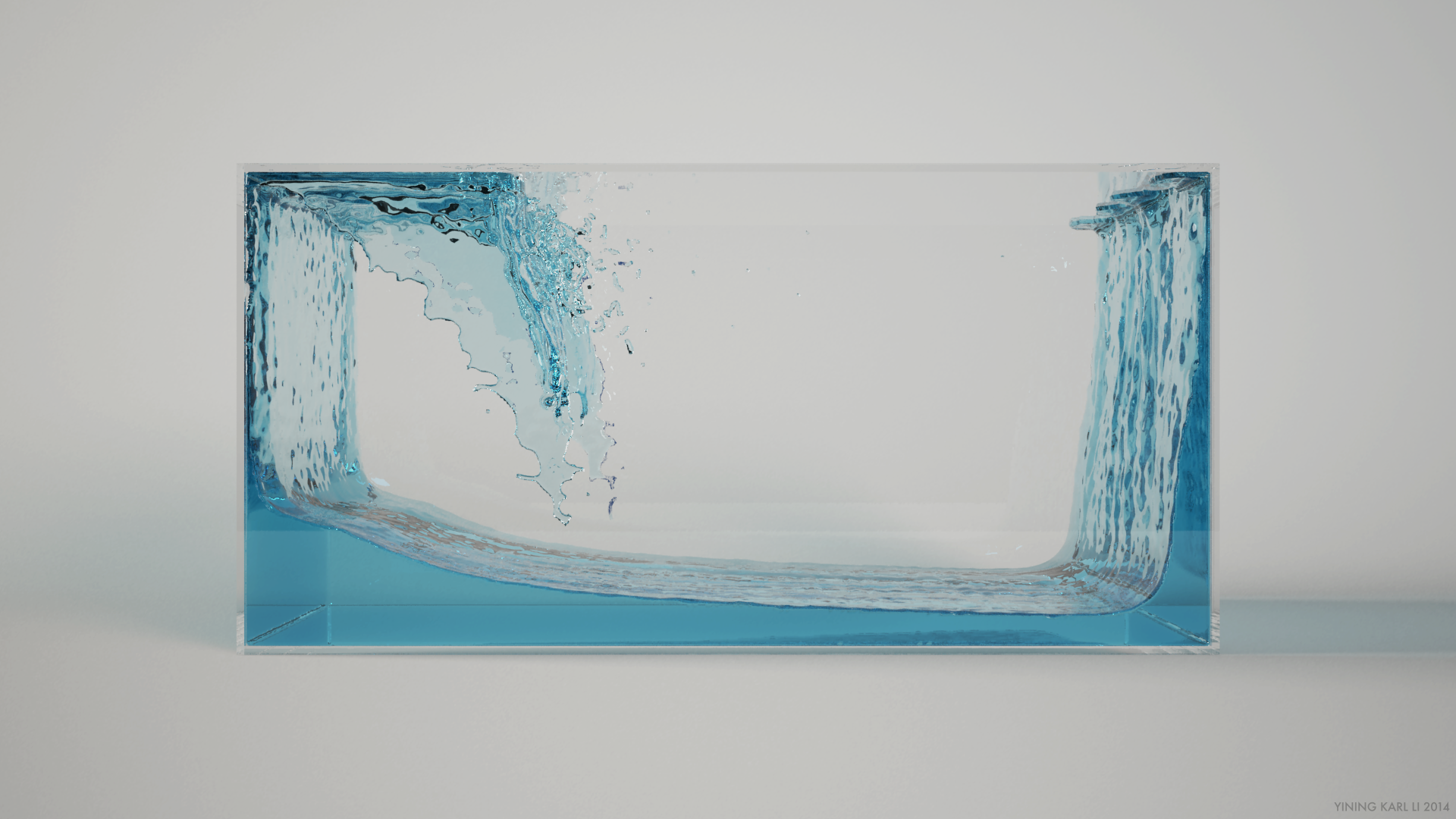
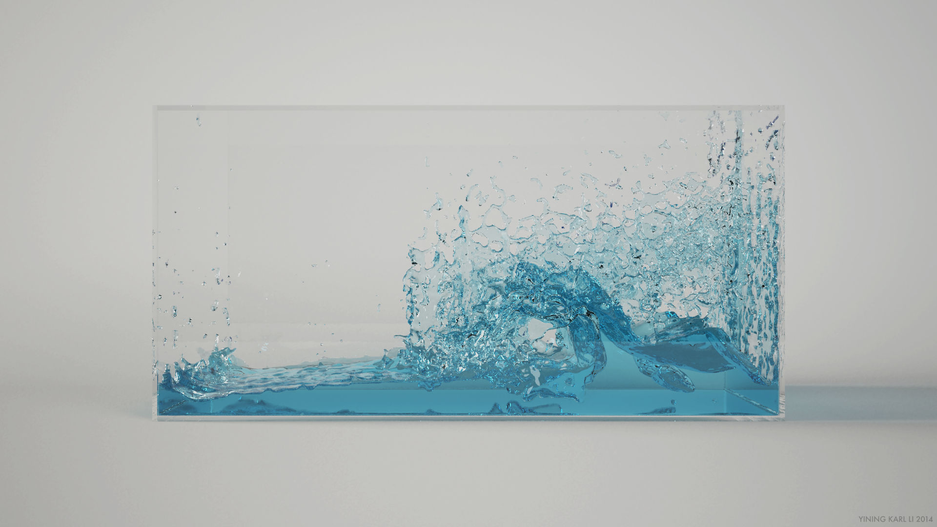
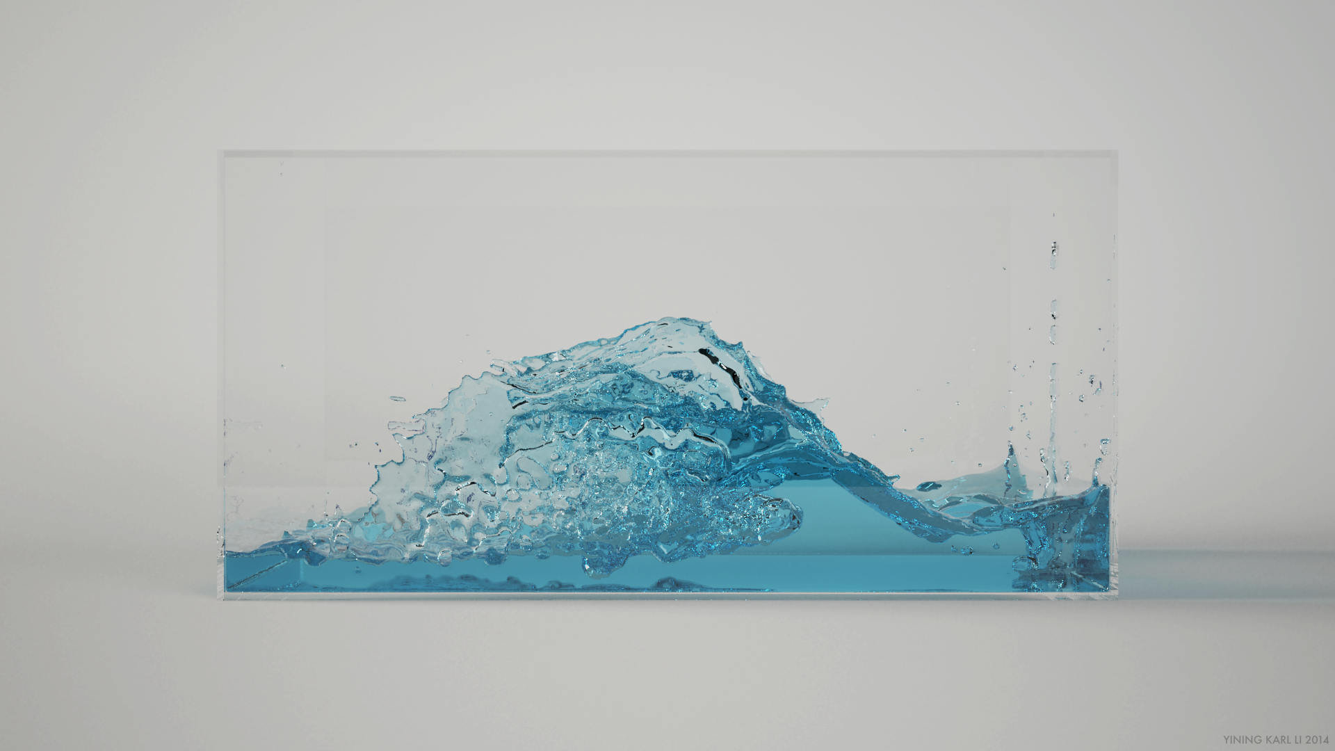
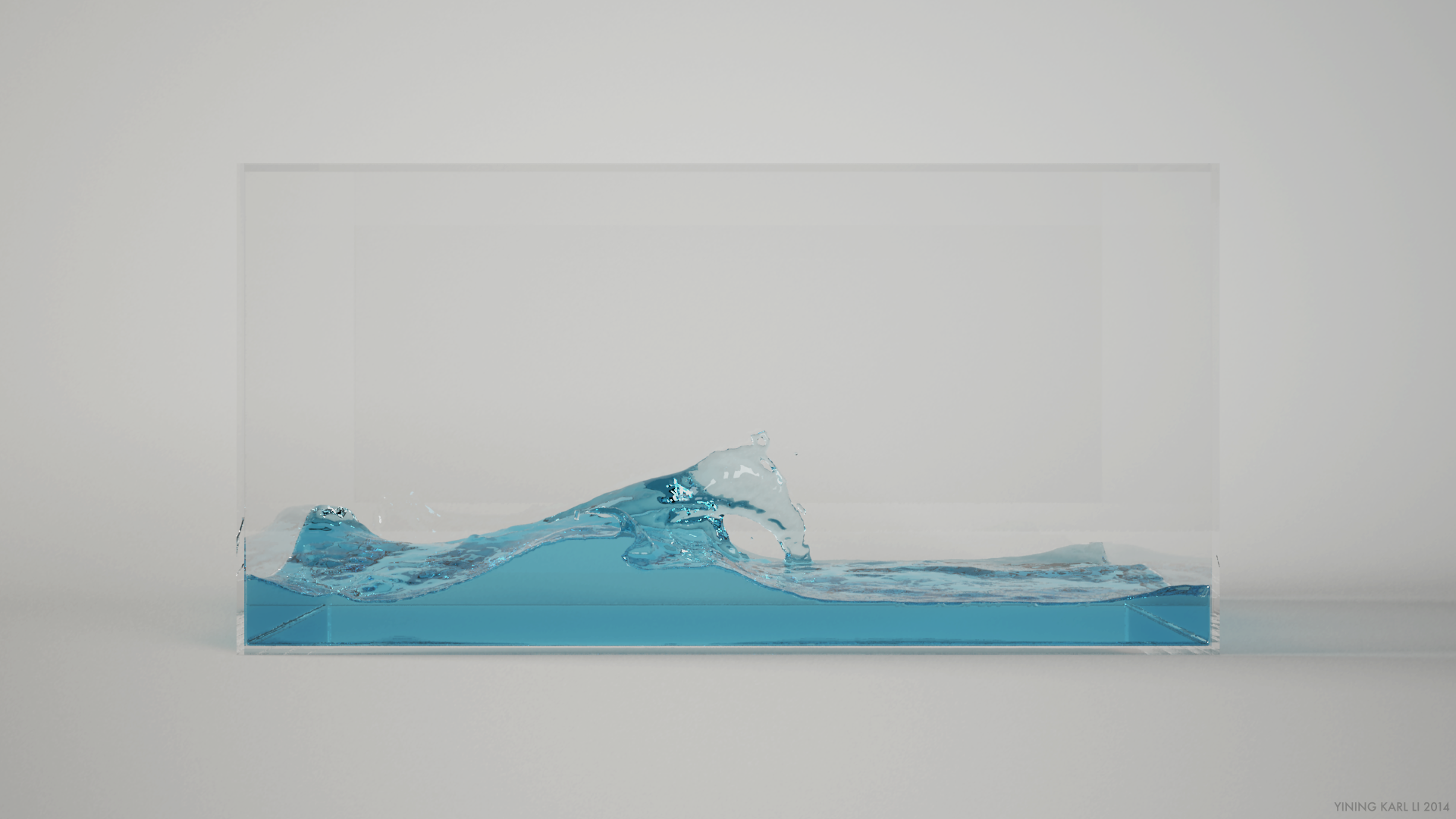
This time around, I’ve tried to build a new meshing/rendering pipeline that resolves those problems. My new meshing/rendering pipeline produces stable, detailed meshes that fit correctly into solid boundaries, all with minimal or no flickering. The following video is the same “dambreak” test from my previous test, but fully meshed and rendered using Vray:
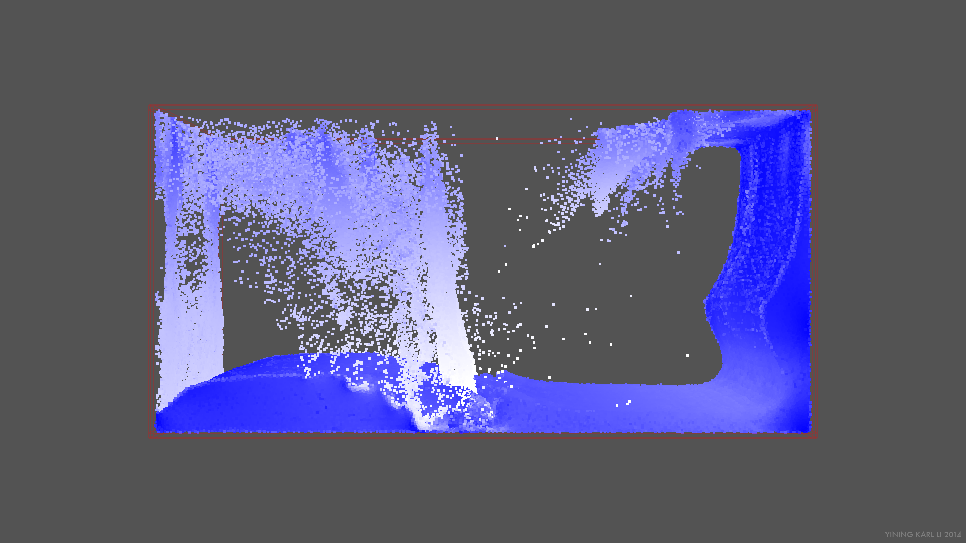
One of the main issues with the old meshing approach was that marching cubes was run directly on the same level set we were using for the simulation, which meant that the resolution of the final mesh was effectively bound to the resolution of the fluid. In a pure semi-Lagrangian simulator, this coupling makes sense, however, in a PIC/FLIP simulator, the resolution of the simulator is dependent on the particle count and not the projection step grid resolution. This property means that even on a simulation with a grid size of 128x64x64, extremely high resolution meshes should be possible if there are enough particles, as long as a level set was constructed directly from the particles completely independently of the projection step grid dimensions.
Fortunately, OpenVDB comes with an enormous toolkit that includes tools for constructing level sets from various type of geometry, including particles, and tools for adaptive level set meshing. OpenVDB also comes with a number of level set operators that allow for artistic tuning of level sets, such as tools for dilating, eroding, and smoothing level set. At the SIGGRAPH 2013 OpenVDB course, Dreamworks had a presentation on how they used OpenVDB’s level set operator tools to extract really nice looking, detailed fluid meshes from relatively low resolution simulations. I also integrated Walt Disney Animation Studios’ Partio library for exporting particle data to standard formats so that I could get particles, level sets, and meshes.
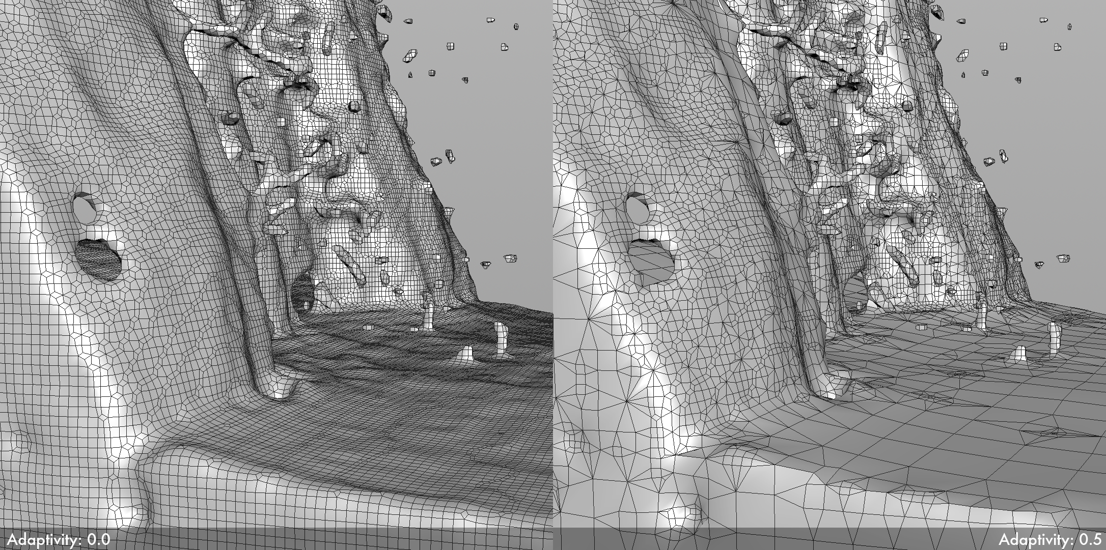
I started by building support for OpenVDB’s adaptive level set meshing directly into my simulator and dumping out OBJ sequences straight to disk. In order to save disk space, I enabled fairly high adaptivity in the meshing. However, upon doing a first render test, I discovered a problem: since OpenVDB’s adaptive meshing optimizes the adaptivity per frame, the result is not temporally coherent with respect to mesh resolution. By itself this property is not a big deal, but it makes reconstructing temporally coherent normals difficult, which can contribute to flickering in final rendering. So, I decided that disk space was not as big deal and just disabled adaptivity in OpenVDB’s meshing for smaller simulations; in sufficiently large sims, the scale of the final render more often than not will make normal issues far less important and disk resource demands become much greater, so the tradeoffs of adaptivity become more worthwhile.
The next problem was getting a stable, fitted liquid-solid interface. Even with a million particles and a 1024x512x512 level set driving mesh construction, the produced fluid mesh still didn’t fit the solid boundaries of the sim precisely. The reason is simple: level set construction from particles works by treating each particle as a sphere with some radius and then unioning all of the spheres together. The first solution I thought of was to dilate the level set and then difference it with a second level set of the solid objects in the scene. Since Houdini has full OpenVDB support and I wanted to test this idea quickly with visual feedback, I prototyped this step in Houdini instead of writing a custom tool from scratch. This approach wound up not working well in practice. I discovered that in order to get a clean result, the solid level set needed to be extremely high resolution to capture all of the detail of the solid boundaries (such as sharp corners). Since the output levelset from VDB’s difference operator has to match the resolution of the highest resolution input, that meant the resultant liquid level set was also extremely high resolution. On top of that, the entire process was extremely slow, even on smaller grids.
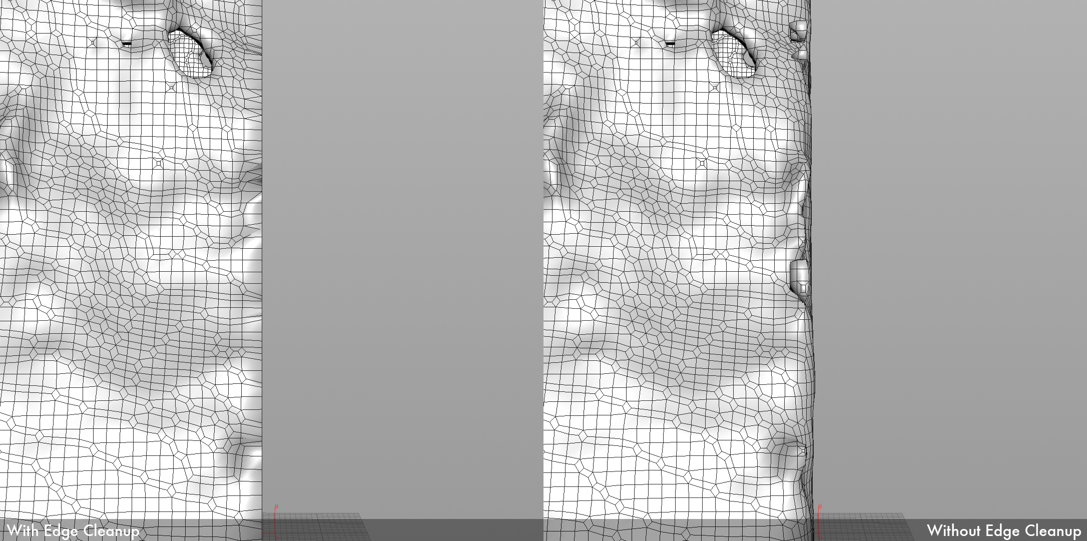
The solution I wound up using was to process the mesh instead of the level set, since the mesh represents significantly less data and at the end of the day the mesh is what we want to have a clean liquid-solid interface. The solution is from every vertex in the liquid mesh, raycast to find the nearest point on the solid boundary to each vertex (this can be done either stochastically, or a level set version of the solid boundary can be used to inform a good starting direction). If the closest point on the solid boundary is within some epsilon distance of the vertex, move the vertex to be at the solid boundary. Obviously, this approach is far simpler than attempting to difference level sets, and it works pretty well. I prototyped this entire system in Houdini.
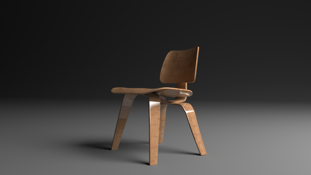
For rendering, I used Vray’s ply2mesh utility to dump the processed fluid meshes directly to .vrmesh files and rendered the result in Vray using pure brute force pathtracing to avoid flickering from temporally incoherent irradiance caching. The final result is the video at the top of this post!
Here are some still frames from the same simulation. The video was rendered with motion blur, these stills do not have any motion blur.