The last assignment of the year for CIS460/560 (I’m still not sure what I’m supposed to call that class) is the dreaded RAYTRACER ASSIGNMENT.

The assignment is actually pretty straightforward: implement a recursive, direct lighting only raytracer with support for Blinn-Phong shading and support for basic primitive shapes (spheres, boxes, and polygon extrusions). In other words, pretty much a barebones implementation of the original Turner Whitted raytracing paper.

I’ve been planning on writing a global-illumination renderer (perhaps based on pathtracing or photon mapping?) for a while now, so my own personal goal with the raytracer project was to use it as a testbed for some things that I know I will need for my GI renderer project. With that in mind, I decided from the start that my raytracer should support rendering OBJ meshes and include some sort of acceleration system for OBJ meshes.

The idea behind the acceleration system goes like this: in the raytracer, one obviously needs to cast rays into the scene and track how they bounce around to get a final image. That means that every ray needs to have intersection tests against objects in the scene in order to determine what ray is hitting what object. Intersection testing against mathematically defined primitives is simple, but OBJ meshes present more of a problem; since an OBJ mesh is composed of a bunch of triangles or polygons, the naive way to intersection test against an OBJ mesh is to check for ray intersections with every single polygon inside of the mesh. This naive approach can get extremely expensive extremely quickly, so a better approach would be to use some sort of spatial data structure to quickly figure out what polygons are within the vicinity of the ray and therefore need intersection testing.

After talking with Joe and trawling around on Wikipedia for a while, I picked a KD-Tree as my spatial data structure for accelerated mesh intersection testing. I won’t go into the details of how KD-Trees work, as the Wikipedia article does a better job of it than I ever could. I will note, however, that the main resources I ended up pulling information from while looking up KD-Tree stuff are Wikipedia, Jon McCaffrey’s old CIS565 slides on spatial data structure, and the fantastic PBRT book that Joe pointed me towards.

Implementing the KD-Tree for the first time took me the better part of two weeks, mainly because I was misunderstanding how the surface area splitting heuristic works. Unfortunately, I probably can’t post actual code for my raytracer, since this is a class assignment that will repeated in future incarnations of the class. However, I can show images!

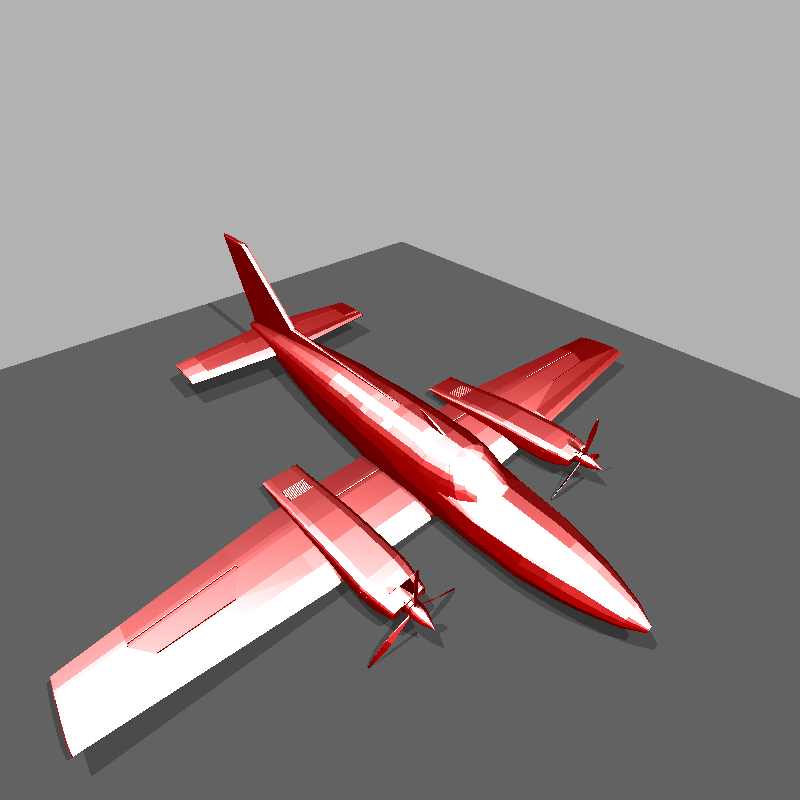
The KD-Tree meant I could render meshes in a reasonable amount of time, so I rendered an airplane:

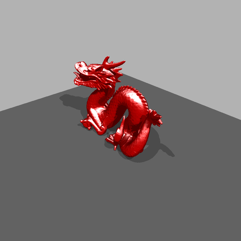
The airplane took about a minute or so to render, which got me wondering how well my raytracer would work if I threw the full 500000+ poly Stanford Dragon at it. This render took about five or six minutes to finish (without the KD-Tree in place, this same image takes about 30 minutes to render):

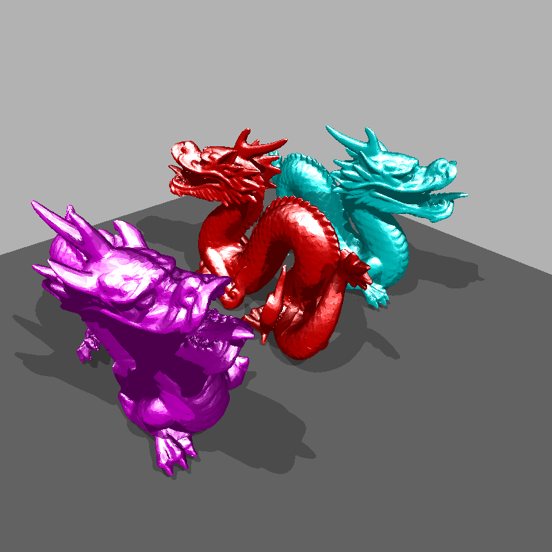
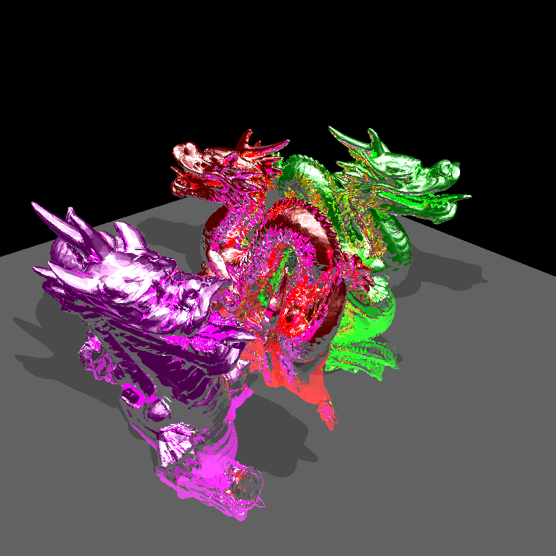
Of course, the natural place to go after one dragon is three dragons. Three dragons took about 15 minutes to render, which is pretty much exactly a three-fold increase over one dragon. That means my renderer’s performance scales more or less linearly, which is good.

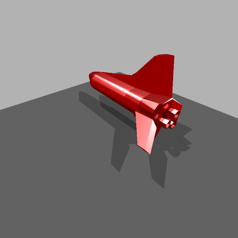
For fun, and because I like space shuttles, here is a space shuttle. Because the space shuttle has a really low poly count, this image took under a minute to render:

For reflections, I took a slightly different approach from the typical recursive method. The normal recursive approach to a raytracer is to begin with one ray, and trace that ray completely through recursion to its recursion depth limit before moving onto the next pixel and ray. However, such an approach might not actually be idea in a GI renderer. For example, from what I understand, in pathtracing a better raytracing approach is to actually trace everything iteratively; that is, trace the first bounce for all rays and store where the rays are, then trace the second bounce for all rays, then the third, and so on and so forth. Basically, such an approach allows one to set an unlimited trace depth and just let the renderer trace and trace and trace until one stops the renderer, but the corresponding cost of such a system is slightly higher memory usage, since ray positions need to be stored for the previous iteration.

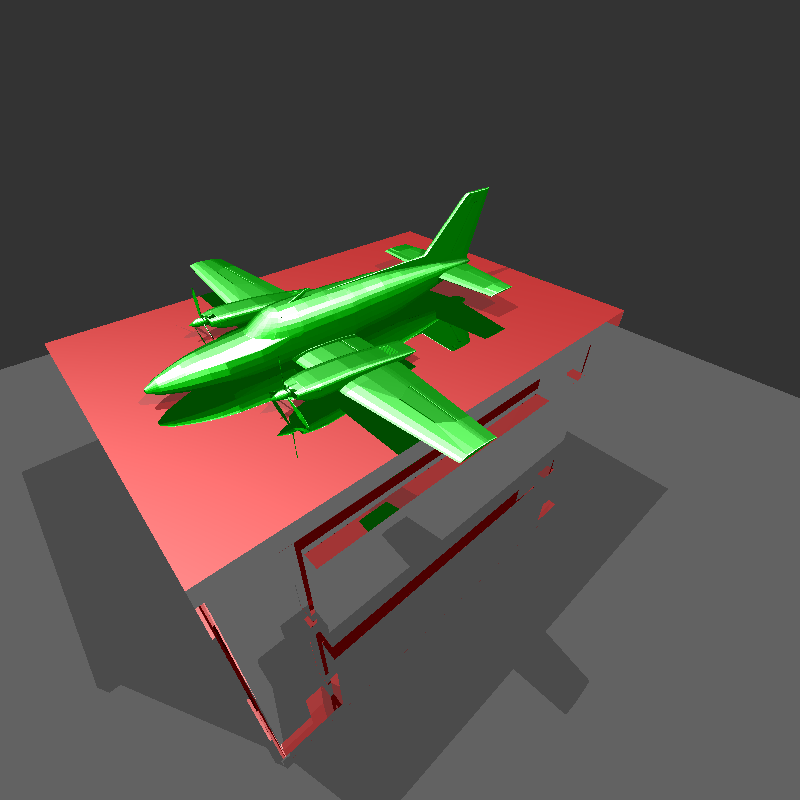
Adding reflections did impact my render times pretty dramatically. I have a suspicion that both my intersection code and my KD-Tree are actually far from ideal, but I’ll have to look at that later. Here’s a test with reflections with the airplane:

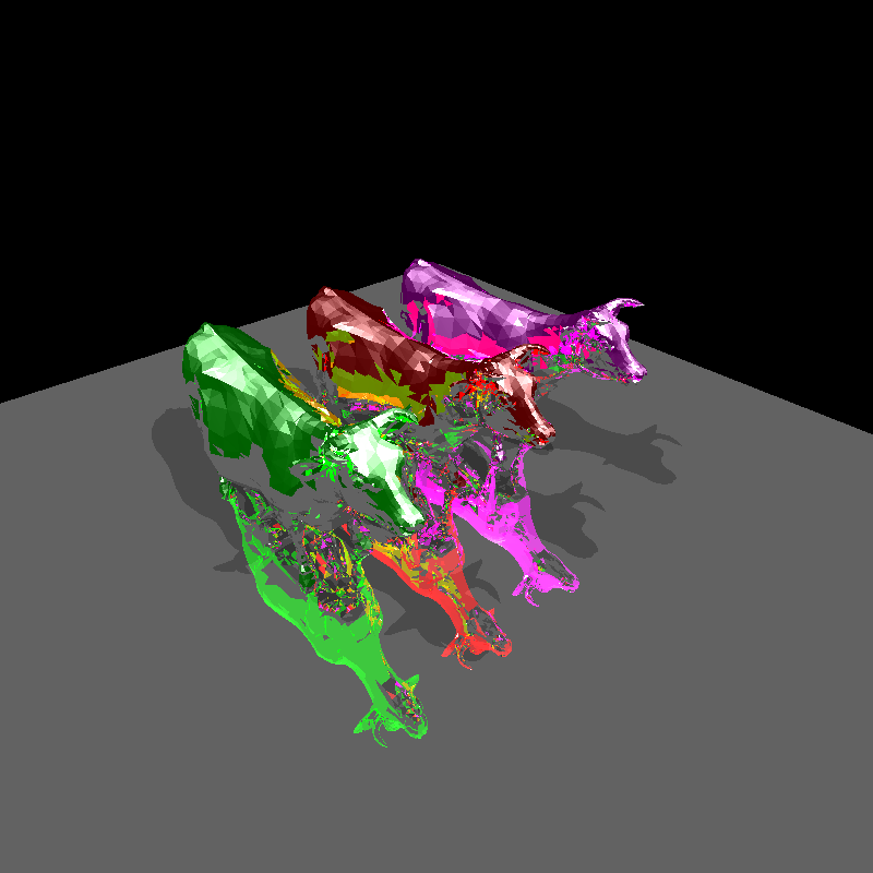
…and here is a test with three reflective dragons. This image took foooorrreeevvveeeerrrr to render…. I actually do not know how long, as I let it run overnight:

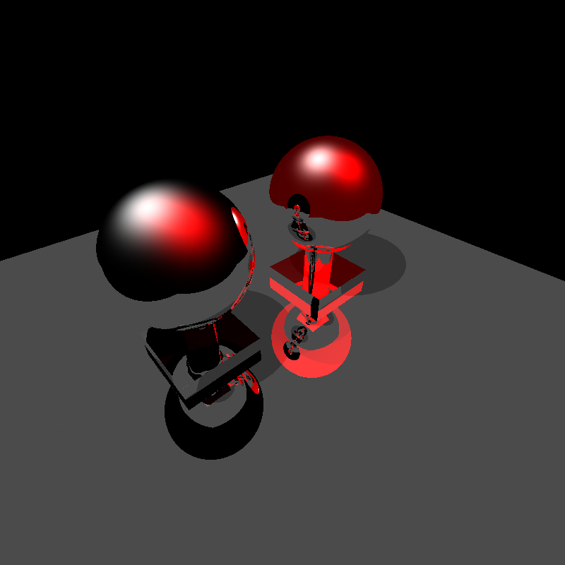
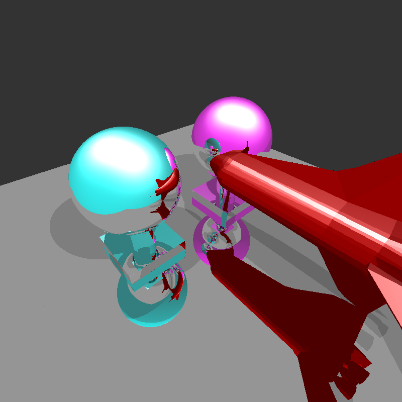
I also added support for multiple lights with varying color support:

Here are some more images rendered with my raytracer:

In conclusion, the raytracer was a fun final project. I don’t think my raytracer is even remotely suitable for actual production use, and I don’t plan on using it for any future projects (unlike my volumetric renderer, which I think I will definitely be using in the future). However, I will definitely be using stuff I learned from the raytracer in my future GI renderer project, such as the KD-tree stuff and the iterative raytracing method. I will probably have to give my KD-tree a total rewrite, since it is really really far from optimal here, so that is something I’ll be starting over winter break! Next stop, GI renderer, CIS563, and CIS565!

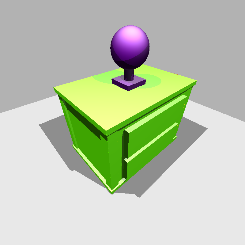
As an amusing parting note, here is the first proper image I ever got out of my raytracer. Awww yeeeaaahhhhhh: