Bidirectional Pathtracing Integrator
As part of Takua a0.5’s complete rewrite, I implemented the vertex connection and merging (VCM) light transport algorithm. Implementing VCM was one of the largest efforts of this rewrite, and is probably the single feature that I am most proud of. Since VCM subsumes bidirectional pathtracing and progressive photon mapping, I also implemented Veach-style bidirectional pathtracing (BDPT) with multiple importance sampling (MIS) and Toshiya Hachisuka’s stochastic progressive photon mapping (SPPM) algorithm. Since each one of these integrators is fairly complex and interesting by themselves, I’ll be writing a series of posts on my BDPT and SPPM implementations before writing about my full VCM implementation. My plan is for each integrator to start with a longer post discussing the algorithm itself and show some test images demonstrating interesting properties of the algorithm, and then follow up with some shorter posts detailing specific tricky or interesting pieces and also show some pretty real-world production-plausible examples of when each algorithm is particularly useful.
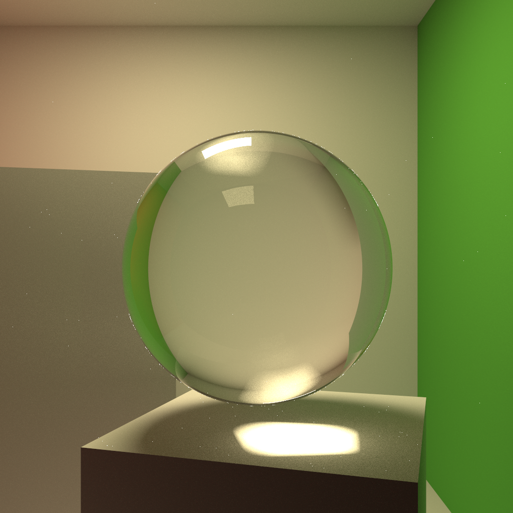
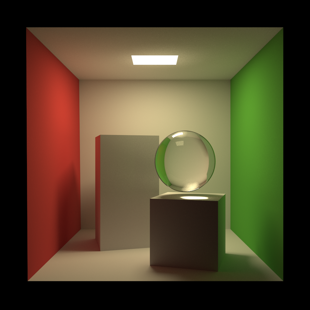
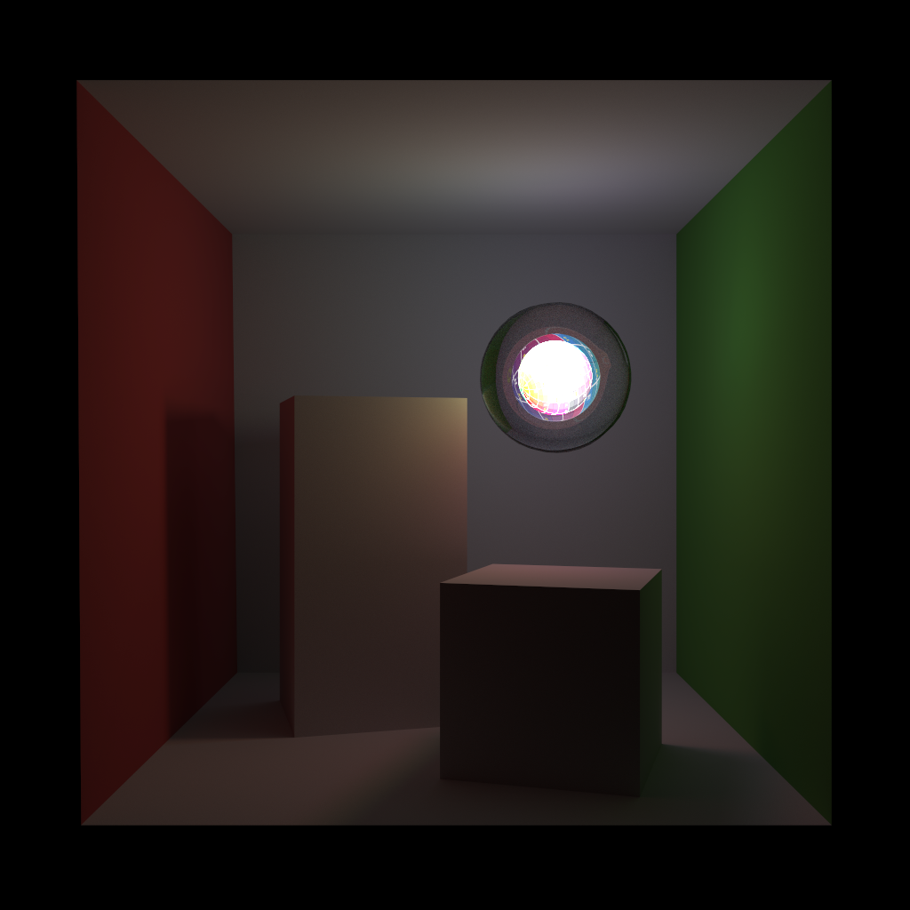
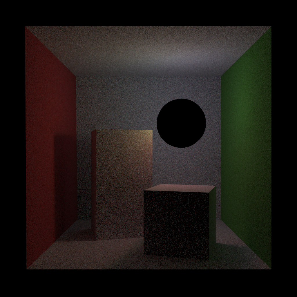
As usual, we’ll start off with an image. Of course, all images in this post are rendered entirely using Takua a0.5. The following image is a Cornell Box lit by a textured sphere light completely encased in a glass sphere, rendered using my bidirectional pathtracer integrator. For reasons I’ll discuss a bit later in this post, this scene belongs to a whole class of scenes that unidirectional pathtracing is absolutely abysmal; these scenes require a bidirectional integrator to converge in any reasonable amount of time:
To understand why BDPT is a more robust integrator than unidirectional pathtracing, we need to start by examining the light transport equation and its path integral formulation. The light transport equation was introduced by Kajiya and is typically presented using the formulation from Eric Veach’s thesis:
Put into words instead of math, the light transport equation simply states that the amount of light leaving any point is equal to the amount of light emitted at that point plus the total amount of light arriving at that point from all directions, weighted by the surface reflectance and absorption at that point. Combined with later extensions to account for effects such as volume scattering and subsurface scattering and diffraction, the light transport equation serves as the basis for all of modern physically based rendering. In order to solve the light transport equation in a practical manner, Veach presents the path integral formulation of light transport:
The path integral states that for a given pixel on an image, the amount of radiance arriving at that pixel is the integral of all radiance coming in through all paths in path space, where a path is the route taken by an individual photon from the light source through the scene to the camera/eye/sensor, and path space simply encompasses all possible paths. Since there is no closed form solution to the path integral, the goal of modern physically based ray-tracing renderers is to sample a representative subset of path space in order to produce a reasonably accurate estimate of the path integral per pixel; progressive renderers estimate the path integral piece by piece, producing a better and better estimate of the full integral with each new iteration.
At this point, we should take a brief detour to discuss the terms “unbiased” versus “biased” rendering. Within the graphics world, there’s a lot of confusion and preconceptions about what each of these terms mean. In actuality, an unbiased rendering algorithm is simply one where each iteration produces an exact result for the particular piece of path space being sampled. A biased rendering algorithm is one where at each iteration, an approximate result is produced for the piece of path space being sampled. However, biased algorithms are not necessarily a bad thing; a biased algorithm can be consistent, that is, converges in the limit to the same result as an unbiased algorithm. Consistency means that an estimator arrives at the accurate result in the limit; so in practice, we should care less about whether or not an algorithm is biased or unbiased so long as it is consistent. BDPT is an unbiased, consistent integrator whereas SPPM is a biased but still consistent integrator.
Going back to the path integral, we can quickly see where unidirectional pathtracing comes from once we view light transport through the path integral. The most obvious way to evaluate the path integral is to do exactly as the path integral says: trace a path starting from a light source, through the scene, and if the path eventually hits the camera, accumulate the radiance along the path. This approach is one form of unidirectional pathtracing that is typically referred to as light tracing (LT). However, since the camera is a fairly small target for paths to hit, unidirectional pathtracing is typically implemented going in reverse: start each path at the camera, and trace through the scene until each path hits a light source or goes off into empty space and is lost. This approach is called backwards pathtracing and is what people usually are referring to when they use the term pathtracing (PT).
As I discussed a few years back in a previous post, pathtracing with direct light importance sampling is pretty efficient at a wide variety of scene types. However, pathtracing with direct light importance sampling will fail for any type of path where the light source cannot be directly sampled; we can easily construct a number of plausible, common setups where this situation occurs. For example, imagine a case where a light source is completely enclosed within a glass container, such as a glowing filament within a glass light bulb. In this case, for any pair consisting of a point in space and a point on the light source, the direction vector to hit the light point from the surface point through glass is not just the light point minus the surface point normalized, but instead has to be at an angle such that the path hits the light point after refracting through glass. Without knowing the exact angle required to make this connection beforehand, the probability of a random direct light sample direction arriving at the glass interface at the correct angle is extremely small; this problem is compounded if the light source itself is very small to begin with.
Taking the sphere light in a glass sphere scene from earlier, we can compare the result of pathtracing without glass around the light versus with glass around the light. The following comparison shows 16 iterations each, and we can see that the version with glass around the light is significantly less converged:
Generally, pathtracing is terrible at resolving caustics, and the glass-in-light scenario is one where all illumination within the scene is through caustics. Conversely, light tracing is quite good at handling caustics and can be combined with direct sensor importance sampling (same idea as direct light importance sampling, just targeting the camera/eye/sensor instead of a light source). However, light tracing in turn is bad at handling certain scenarios that pathtracing can handle well, such as small distant spherical lights.
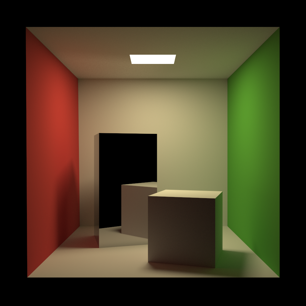
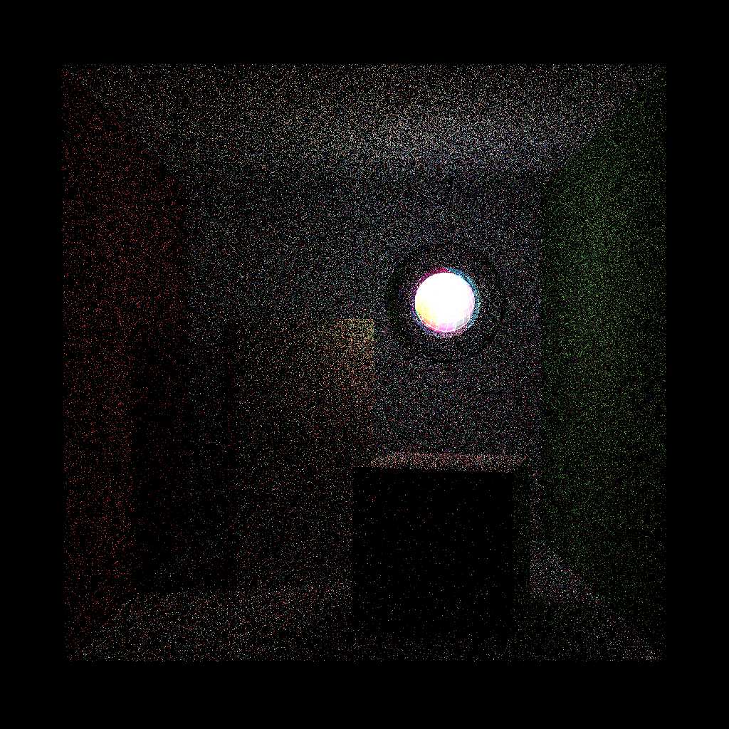
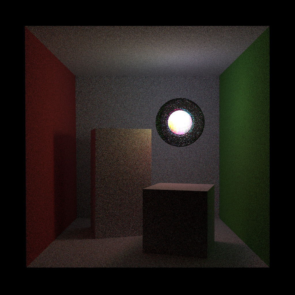
The following image again shows the sphere light in a glass sphere scene, but is now rendered for 16 iterations using light tracing. Note how the render is significantly more converged, for approximately the same computational cost. The glass sphere and sphere light render as black since in light tracing, the camera cannot be directly sampled from a specular surface.
Since bidirectional pathtracing subsumes both pathtracing and light tracing, I implemented pathtracing and light tracing simultaneously and used each integrator as a check on the other, since correct integrators should converge to the same result. Implementing light tracing requires BSDFs and emitters to be a bit more robust than in vanilla pathtracing; emitters have to support both emission and illumination, and BSDFs have to support bidirectional evaluation. Light tracing also requires the ability to directly sample the camera and intersect the camera’s image plane to figure out what pixel to contribute a path to; as such, I implemented a rasterize function for my thin-lens and fisheye camera models. My thin-lens camera’s rasterization function supports the same depth of field and bokeh shape capabilities that the thin-lens camera’s raycast function supports.
The key insight behind bidirectional pathtracing is that since light tracing and vanilla pathtracing each have certain strengths and weaknesses, combining the two sampling techniques should result in a more robust path sampling technique. In BDPT, for each pixel per iteration, a path is traced starting from the camera and a second path is traced starting from a point on a light source. The two paths are then joined into a single path, conditional on an unoccluded line of sight from the end vertices of the two paths to each other. A BDPT path of length k with k+1 vertices can then be used to generate up to k+2 path sampling techniques by connecting each vertex on each subpath to every other vertex on the other subpath. While BDPT per iteration is much more expensive than unidirectional pathtracing, the much larger number of sampling techniques leads to a significantly higher convergence rate that typically outweighs the higher computational cost.
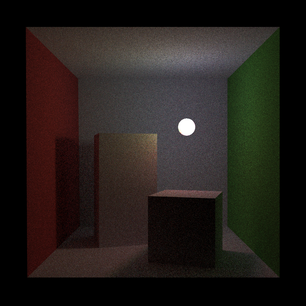
Below is the same scene as above rendered with 16 iterations of BDPT, and rendered with the same amount of computation time (about 5 iterations of BDPT). Note how with just 5 iterations, the BDPT result with the glass sphere has about the same level of noise as the pathtraced result for 16 iterations without the glass sphere. At 16 iterations, the BDPT result with the glass sphere is noticeably more converged than the pathtraced result for 16 iterations without the glass sphere.

A naive implementation of BDPT would be for each pixel per iteration, trace a full light subpath, store the result, trace a full camera subpath, store the result, and then perform the connection operations between each vertex pair. However, since this approach requires storing the entirety of both subpaths for the entire iteration, there is room for some improvement. For Takua a0.5, my implementation stores only the full light subpath. At each bounce of the camera subpath, my implementation connects the current vertex to each vertex of the stored light subpath, weights and accumulates the result, and then moves onto the next bounce without having to store previous path vertices.
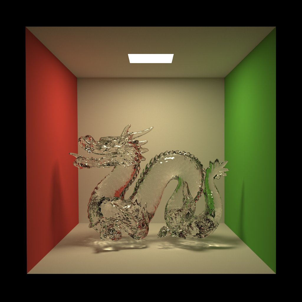
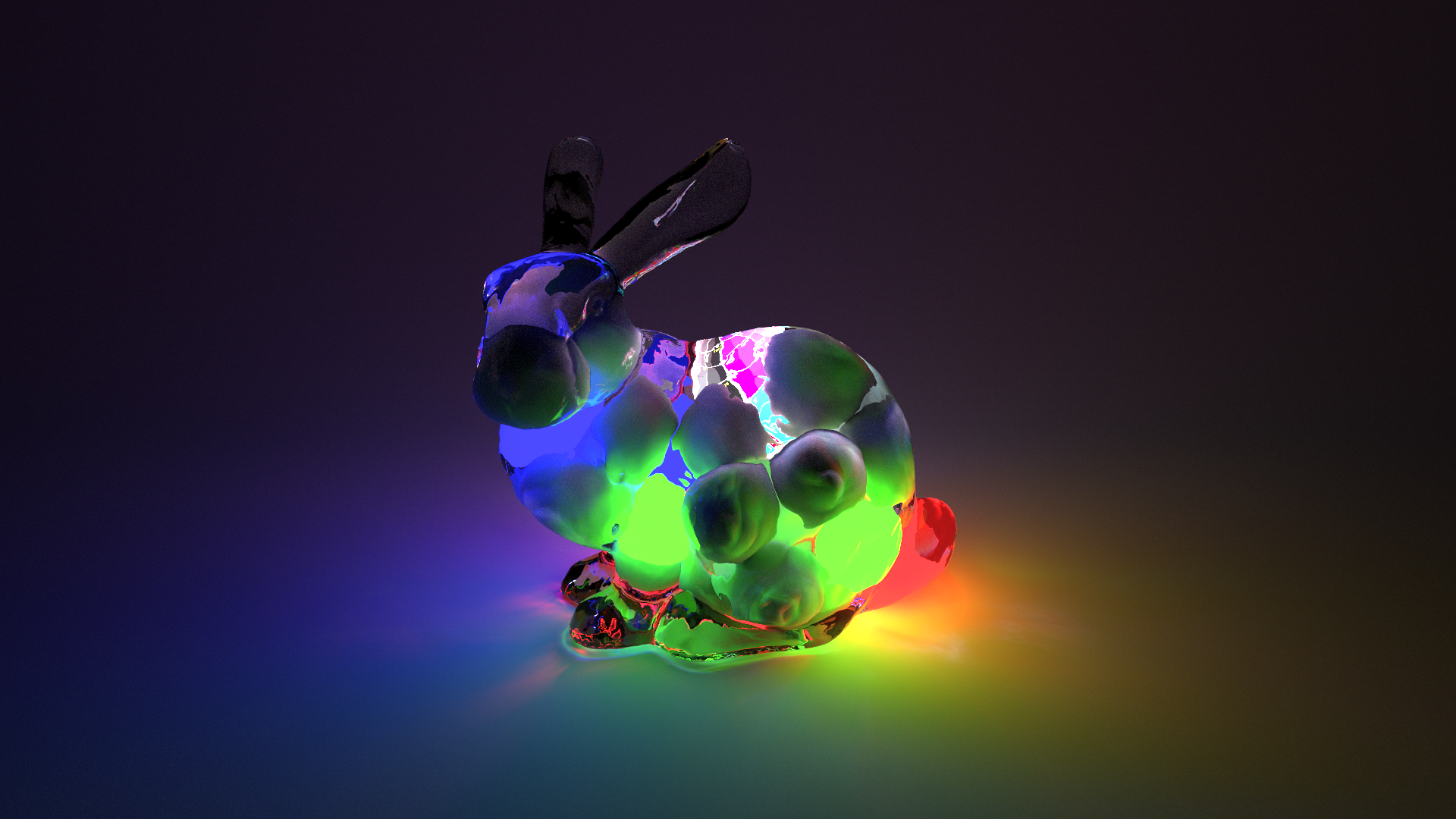
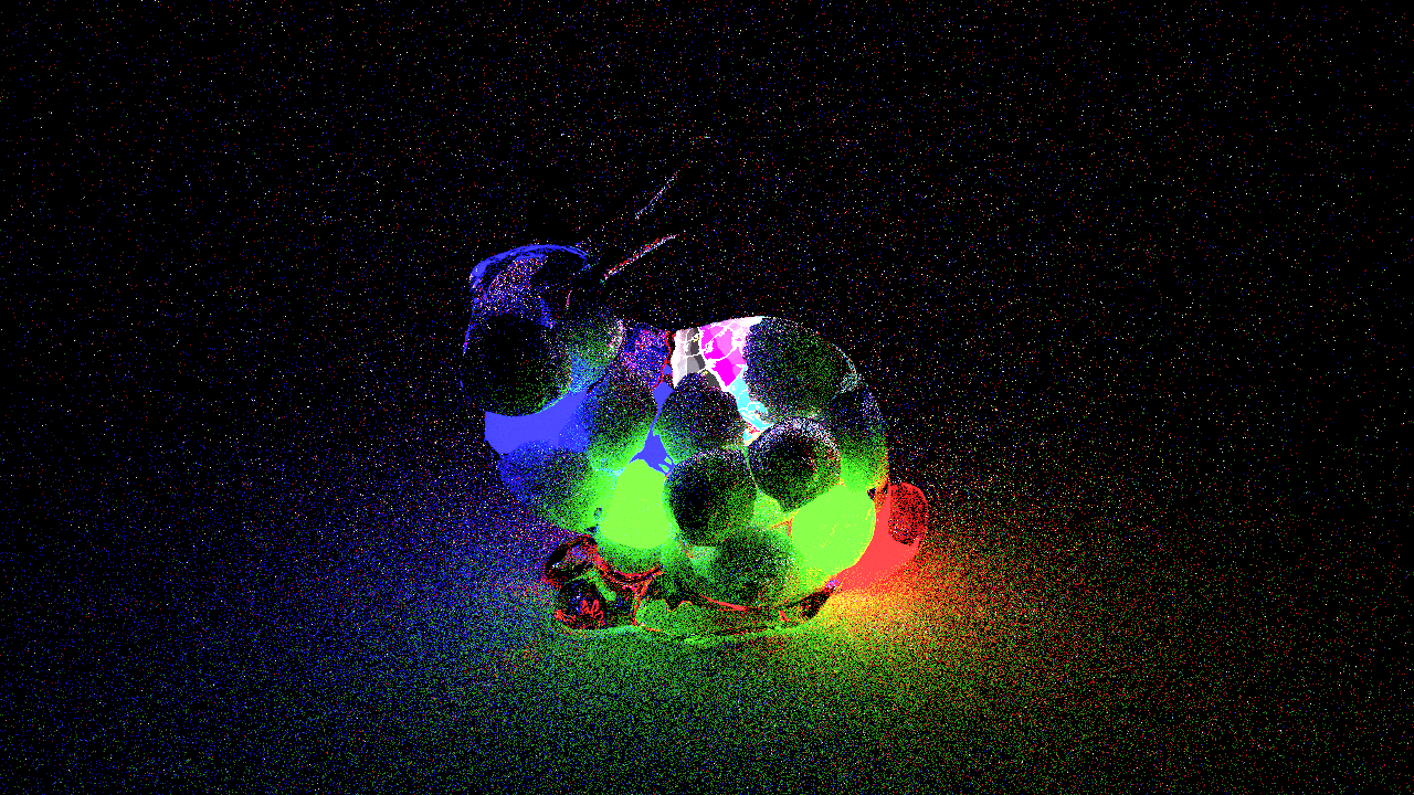
The following image is another example of a scene that BDPT is significantly better at sampling than any unidirectional pathtracing technique. The scene consists of a number of diffuse spheres and spherical lights inside of a glass bunny. In this scene, everything outside of the bunny is being lit using only caustics, while diffuse surfaces inside of the bunny are being lit using a combination of direct lighting, indirect diffuse bounces, and caustics from outside of the bunny reflecting/refracting back into the bunny. This last type of lighting belongs to a category of paths known as specular-diffuse-specular (SDS) paths that are especially difficult to sample unidirectionally.
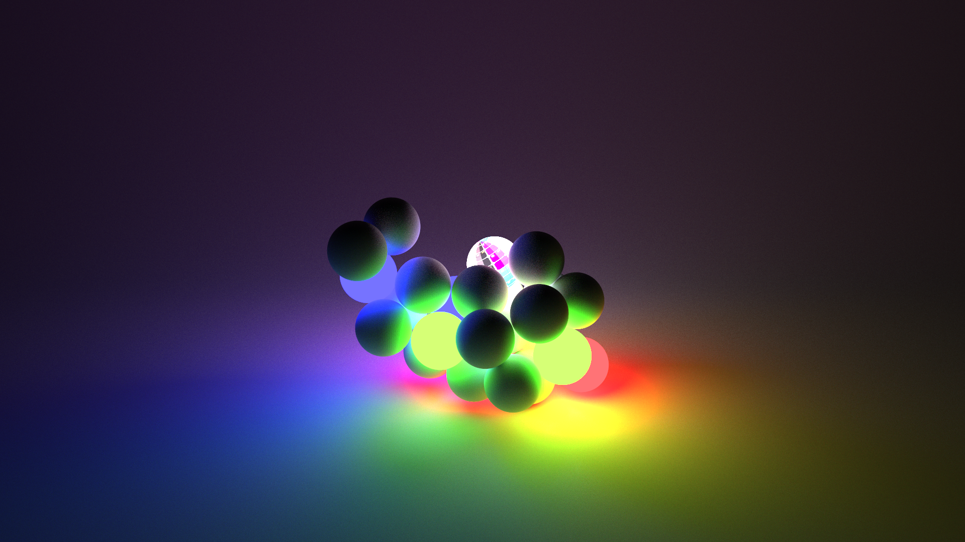
Here is the same scene as above, but with the glass bunny removed just so seeing what is going on with the spheres is a bit easier:
Comparing pathtracer versus BDPT performance for 16 interations, BDPT’s vastly better performance on this scene becomes obvious:

In the next post, I’ll write about multiple importance sampling (MIS), how it impacts BDPT, and my MIS implementation in Takua a0.5.