Porting Takua Renderer to 64-bit ARM- Part 1
Table of Contents
Introduction
For almost its entire existence my hobby renderer, Takua Renderer, has built and run on Mac, Windows, and Linux on x86-64. I maintain Takua on all three major desktop operating systems because I routinely run and use all three operating systems, and I’ve found that building with different compilers on different platforms is a good way for making sure that I don’t have code that is actually wrong but just happens to work because of the implementation quirks of a particular compiler and / or platform. As of last year, Takua Renderer now also runs on 64-bit ARM, for both Linux and Mac! 64-bit ARM is often called either aarch64 or arm64; these two terms are interchangeable and mean the same thing (aarch64 is the official name for 64-bit ARM and is what Linux tends to use, while arm64 is the name that Apple and Microsoft’s tools tend to use). For the sake of consistency, I’ll use the term arm64.
This post is the first of a two-part writeup of the process I undertook to port Takua Renderer to run on arm64, along with interesting stuff that I learned along the way. In this first part, I’ll write about motivation and the initial port I undertook in the spring to arm64 Linux (specifically Fedora). I’ll also write about how arm64 and x86-64’s memory ordering guarantees differ and what that means for lock-free code, and I’ll also do some deeper dives into topics such as floating point differences between different processors and a case study examining how code compiles to x86-64 versus to arm64. In the second part, I’ll write about porting to arm64-based Apple Silicon Macs and I’ll also write about getting Embree up and running on ARM, creating Universal Binaries, and some other miscellaneous topics.
Motivation
So first, a bit of a preamble: why port to arm64 at all? Today, basically most, if not all, of the animation/VFX industry renders on x86-64 machines (and a vast majority of those machines are likely running Linux), so pretty much all contemporary production rendering development happens on x86-64. However, this has not always been true! A long long time ago, much of the computer graphics world was based on MIPS hardware running SGI’s IRIX Unix variant; in the early 2000s, as SGI’s custom hardware began to fall behind the performance-per-dollar, performance-per-watt, and even absolute performance that commodity x86-based machines could offer, the graphics world undertook a massive migration to the current x86 world that we live in today. Apple undertook a massive migration from PowerPC to x86 in the mid/late 2000s for similar reasons.
At this point, an ocean of text has been written about why it is that x86 (and by (literal) extension x86-64) became the dominant ISA in desktop computing and in the server space. One common theory that I like is that x86’s dominance was a classic example of disruptive innovation from the low end. A super short summary of disruptive innovation from the low end is that sometimes, a new player enters an existing market with a product that is much less capable but also much cheaper than existing competing products. By being so much cheaper, the new product can generate a new, larger market that existing competing products can’t access due to their higher cost or different set of requirements or whatever. As a result, the new product gets massive investment since the new product is the only thing that can capture this new larger market, and in turn this massive influx of investment allows the new player to iterate faster and rapidly grow its product in capabilities until the new player becomes capable of overtaking the old market as well. This theory maps well to x86; x86-based desktop PCs started off being much cheaper but also much less capable than specialized hardware such as SGI machines, but the investment that poured into the desktop PC space allowed x86 chips to rapidly grow in absolute performance capability until they were able to overtake specialized hardware in basically every comparable metric. At that point, moving to x86 became a no-brainer for many industries, including the computer graphics realm.
I think that ARM is following the same disruptive innovation path that x86 did, only this time the starting “low end” point is smartphones and tablets, which is an even lower starting point than desktop PCs were. More importantly, I think we’re now at a tipping point for ARM. For many years now, ARM chips have offered better performance-per-dollar and performance-per-watt than any x86-64 chip from Intel or AMD, and the point where arm64 chips can overtake x86-64 chips in absolute performance seems plausibly within sight over the next few years. Notably, Amazon’s in-house Graviton2 arm64 CPU and Apple’s M1 arm64-based Apple Silicon chip are both already highly competitive in absolute performance terms with high end consumer x86-64 CPUs, while consuming less power and costing less. Actually, I think that this trend should have been obvious to anyone paying attention to Apple’s A-series chips since the A9 chip was released in 2015.
In cases of disruptive innovation from the low end, the outer edge of the absolute high end is often the last place where the disruption reaches. One of the interesting things about the high-end rendering field is that high-end rendering is one of a relatively small handful of applications that sits at the absolute outer edge of high end compute performance. All of the major animation and VFX studios have render farms (either on-premises or in the cloud) with core counts somewhere in the tens of thousands of cores; these render farms have more similarities with supercomputers than they do with a regular consumer desktop or laptop. I don’t know that anyone has actually tried this, but my guess is that if someone benchmarked any major animation or VFX studio’s render farm using the LINPACK supercomputer benchmark, the score would sit very respectably somewhere in the upper half of the TOP500 supercomputer list. With the above in mind, the fact that the fastest supercomputer in the world is now an arm64-based system should be an interesting indicator of where ARM is now in the process of catching up to x86-64 and how seriously all of us in high-end computer graphics should be when contemplating the possibility of an ARM-based future.
So all of the above brings me to why I undertook porting Takua to arm64. The reason is because I think we can now plausibly see a potential near future in which the fastest, most efficient, and most cost effective chips in the world are based on arm64 instead of x86-64, and the moment this potential future becomes reality, high-performance software that hasn’t already made the jump will face growing pressure to port to arm64. With Apple’s in-progress shift to arm64-based Apple Silicon Macs, we may already be at this point. I can’t speak for any animation or VFX studio in particular; everything I have written here is purely personal opinion and personal conjecture, but I’d like to be ready in the event that a move to arm64 becomes something we have to face as an industry, and what better way is there to prepare than to try with my own hobby renderer first! Also, for several years now I’ve thought that Apple eventually moving Macs to arm64 was obvious given the progress the A-series Apple chips were making, and since macOS is my primary personal daily use platform, I figured I’d have to port Takua to arm64 eventually anyway.
Porting to arm64 Linux
I actually first attempted an ARM port of Takua several years ago, when Fedora 27 became the first version of Fedora to support arm64 single-board computers (SBCs) such as the Raspberry Pi 3B or the Pine A64. I’ve been a big fan of the Raspberry Pi basically since the original first came out, and the thought of porting Takua to run on a Raspberry Pi as an experiment has been with me basically since 2012. However, Takua is written very much with 64-bit in mind, and the first two generations of Raspberry Pis only had 32-bit ARMv7 processors. I actually backed the original Pine A64 on Kickstarter in 2015 precisely because it was one of the very first 64-bit ARMv8 boards on the market, and if I remember correctly, I also ordered the Raspberry Pi 3B the week it was announced in 2016 because it was the first 64-bit ARMv8 Raspberry Pi. However, my Pine A64 and Raspberry Pi 3B mostly just sat around not doing much because I was working on a bunch of other stuff, but that actually wound up working out because by the time I got back around to tinkering with SBCs in late 2017, Fedora 27 had just been released. Thanks to a ton of work from Peter Robinson at Red Hat, Fedora 27 added native arm64 support that basically worked out-of-the-box on both the Raspberry Pi 3B and the Pine A64, which was ideal for me since my Linux distribution of choice for personal hobby projects is Fedora. Since I already had Takua building and running on Fedora on x86-64, being able to use Fedora as the target distribution for arm64 as well meant that I could eliminate different compiler and system library versions as a variable factor; I “just” had to move everything in my Fedora x86-64 build over to Fedora arm64. However, back in 2017, I found that a lot of the foundational libraries that Takua depends on just weren’t quite ready on arm64 yet. The problem usually wasn’t with the actual source code itself, since anything written in pure C++ without any intrinsics or inline assembly should just compile directly on any platform with a supported compiler; instead, the problem was usually just in build scripts not knowing how to handle small differences in where system libraries were located or stuff like that. At the time I was focused on other stuff, so I didn’t try particularly hard to diagnose and work around the problems I ran into; I kind of just shrugged and put it all aside to revisit some other day.
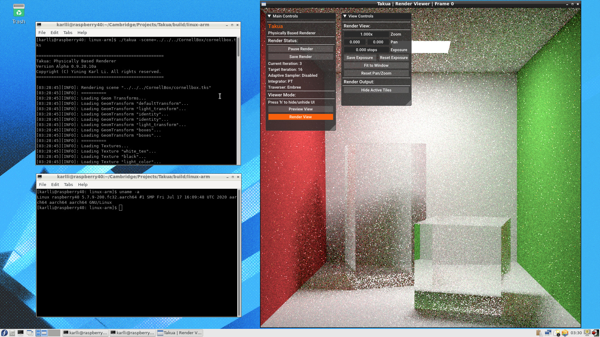
Fast forward to early 2020, when rumors started circulating of a potential macOS transition to 64-bit ARM. As the rumors grew, I figured that this was a good time to return to porting Takua to arm64 Fedora in preparation for if a macOS transition actually happened. I had also recently bought a Raspberry Pi 4B with 4 GB of RAM; the 4 GB of RAM made actually building and running complex code on-device a lot easier than with the Raspberry Pi 3B/3B+’s 1 GB of RAM. By this point, the arm64 build support level for Takua’s dependencies had improved dramatically. I think that as arm64 devices like the iPhone and iPad Pro have gotten more and more powerful processors over the last few years and enabled more and more advanced and complex iOS / iPadOS apps (and similarly with Android devices and Android apps), more and more open source libraries have seen adoption on ARM-based platforms and have seen ARM support improve as a result. Almost everything just built and worked out-of-the-box on arm64, including (to my enormous surprise) Intel’s TBB library! I had assumed that TBB would be x86-64-only since TBB is an Intel project, but it turns out that over the years, the community has contributed support for ARMv7 and arm64 and even PowerPC to TBB. The only library that didn’t work out-of-the-box or with minor changes was Embree, which relies heavily on SSE and AVX intrinsics and has small amounts of inline x86-64 assembly. To get things up and running initially, I just disabled Takua’s Embree-based traversal backend and fell back to my own custom BVH traversal backend. My own custom BVH traversal backend isn’t nearly as fast as Embree and is instead meant to serves as a reference implementation and fallback for when Embree isn’t available, but for the time being since the goal was just to get Takua working at all, losing performance due to not having Embree was fine. As you can see by the “Traverser: Embree” label in Takua Renderer’s UI in Figure 1, I later got Embree up and running on arm64 using Syoyo Fujita’s embree-aarch64 port, but I’ll write more about that in the next post. To be honest, the biggest challenge with getting everything compiled and running was just the amount of patience that was required. I never seem to be able to get cross-compilation for a different architecture right because I always forget something, so instead of cross-compiling for arm64 from my nice big powerful x86-64 Fedora workstation, I just compiled for arm64 directly on the Raspberry Pi 4B. While the Raspberry Pi 4B is much faster than the Raspberry Pi 3B, it’s still nowhere near as fast as a big fancy dual-Xeon workstation, so some libraries took forever to compile locally (especially Boost, which I wish I didn’t have to have a dependency on, but I have to since OpenVDB depends on Boost). Overall getting a working build of Takua up and running on arm64 was very fast; from deciding to undertake the port to getting a first image back took only about a day’s worth of work, and most of that time was just waiting for stuff to compile.
However, getting code to build is a completely different question from getting code to run correctly (unless you’re using one of those fancy proof-solver languages I guess). The first test renders I did with Takua on arm64 Fedora looked fine to my eye, but when I diff’d them against reference images rendered on x86-64, I found some subtle differences; the source of these differences took me a good amount of digging to understand! Chasing this problem down led down some interesting rabbit holes exploring important differences between x86-64 and arm64 that need to be considered when porting code between the two platforms; just because code is written in portable C++ does not necessarily mean that it is always actually as portable as one might think!
Floating Point Consistency (or lack thereof) on Different Systems
Takua has two different types of image comparison based regression tests: the first type of test renders out to high samples-per-pixel numbers and does comparisons with near-converged images, while the second type of test renders out and does comparisons using a single sample-per-pixel. The reason for these two different types of tests is because of how difficult getting floating point calculations to match across different compilers / platforms / processors is. Takua’s single-sample-per-pixel tests are only meant to catch regressions on the same compiler / platform / processor, while Takua’s longer tests are meant to test overall correctness of converged renders. Because of differences in how floating point operations come out on different compilers / platforms / processors, Takua’s convergence tests don’t require an exact match; instead, the tests use small, predefined difference thresholds that comparisons must stay within to pass. The difference thresholds are basically completely ad-hoc; I picked them to be at a level where I can’t perceive any difference when flipping between the images, since I put together my testing system before image differencing systems that formally factor in perception [Andersson et al. 2020] were published. A large part of the differences between Takua’s test results on x86-64 versus arm64 come from these problems with floating point reproducibility across different systems. Because of how commonplace this issue is and how often this issue is misunderstood by programmers who haven’t had to deal with it, I want to spend a few paragraphs talking about floating point numbers.
A lot of programmers that don’t have to routinely deal with floating point calculations might not realize that even though floating point numbers are standardized through the IEEE754 standard, in practice reproducibility is not at all guaranteed when carrying out the same set of floating point calculations using different compilers / platforms / processors! In fact, starting with the same C++ floating point code, determinism is only really guaranteed for successive runs using binaries generated using the same compiler, with the same optimizations enabled, on the same processor family; sometimes running on the same operating system is also a requirement for guaranteed determinism. There are three main reasons [Kreinin 2008] why reproducing exactly the same results from the same set of floating point calculations across different systems is so inconsistent: compiler optimizations, processor implementation details, and different implementations of built-in “complex” functions like sine and cosine .
The first reason above is pretty easy to understand: operations like addition and multiplication are commutative, meaning they can be done in any order, and often a compiler in an optimization pass may choose to reorder commutative math operations.
However, as anyone who has dealt extensively with floating point numbers knows, due to how floating point numbers are represented [Goldberg 1991] the commutative and associative properties of addition and multiplication do not actually hold true for floating point numbers; not even for IEEE754 floating point numbers!
Sometimes reordering floating point math is expressly permitted by the language, and sometimes doing this is not actually allowed by the language but happens anyway in the compiler because the user has specified flags like -ffast-math, which tells the compiler that it is allowed to sacrifice strict IEEE754 and language math requirements in exchange for additional optimization opportunities.
Sometimes the compiler can just have implementation bugs too; here is an example that I found on the llvm-dev mailing lists describing a bug with loop vectorization that impacts floating point consistency!
The end result of all of the above is that the same floating point source code can produce subtly different results depending on which compiler is used and which compiler optimizations are enabled within that compiler.
Also, while some compiler optimization passes operate purely on the AST built from the parser or operate purely on the compiler’s intermediate representation, there can also be optimization passes that take into account the underlying target instruction set and choose to carry out different optimizations depending on the what’s available in the target processor architecture.
These architecture-specific optimizations mean that even the same floating point source code compiled using the same compiler can still produce different results on different processor architectures!
Architecture-specific optimizations are one reason why floating point results on x86-64 versus arm64 can be subtly different.
Also, another fun fact: the C++ specification doesn’t actually specify a binary representation for floating point numbers, so in principle a C++ compiler could outright ignore IEEE754 and use something else entirely, although in practice this is basically never the case since all modern compilers like GCC, Clang, and MSVC use IEEE754 floats.
The second reason floating point math is so hard to reproduce exactly across different systems is in how floating point math is implemented in the processor itself. Differences at this level is a huge source of floating point differences between x86-64 and arm64. In both x86-64 and arm64, at the assembly level individual arithmetic instructions such as add, subtract, multiple, divide, etc all adhere strictly to the IEEE754 standard. However, the IEEE754 standard is itself… surprisingly loosely specified in some areas! For example, the IEEE754 standard specifies that intermediate results should be as precise as possible, but this means that two different implementations of a floating point addition instructions both adhering to IEEE754 can actually produce different results for the same input if they use different levels of increased precision internally. Here’s a bit of a deprecated example that is still useful to know for historical reasons: everyone knows that an IEEE754 floating point number is 32 bits, but older 32-bit x86 specifies that internal calculations be done using 80-bit precision, which is a holdover from the Intel 8087 math coprocessor. Every x86 (and by extension x86-64) processor when using x87 FPU instructions actually does floating point math using 80 bit internal precision and then rounds back down to 32 bit floats in hardware; the 80 bit internal representation is known as the x86 extended precision format. But even within the same x86 processor, we can still get difference floating point results depending on if the compiler has output x87 FPU instructions or SSE instructions; SSE stays within 32 bits at all times, which means SSE and x87 on the same processor doing the same floating point math isn’t guaranteed to produce the exact same answer. Of course, modern x86-64 generally uses SSE for floating point math instead of x87, but different amounts of precision truncation can still happen depending on what order values are loaded into SSE registers and back into other non-SSE registers. Furthermore, SSE is sufficiently under-specified that the actual implementation details can differ, which is why the same SSE floating point instructions can produce different results on Intel versus AMD processors. Similarly, the ARM architecture doesn’t actually specify a particular FPU implementation at all; the internals of the FPU are left up to each processor designer; for example, the VFP/NEON floating point units that ship on the Raspberry Pi 4B’s Cortex-A72-based CPU use up to 64 bits of internal precision [Johnston 2020]. So, while the x87, SSE on Intel, SSE on AMD, and VFP/NEON FPU implementations are IEEE754-compliant, because of their internal maximum precision differences they can still all produce different results from each other. There are many more examples of areas where IEEE754 leaves in wiggle room for different implementations to do different things [Obiltschnig 2006], and in practice different CPUs do use this wiggle room to do things differently from each other. For example, this wiggle room is why for floating point operations at the extreme ends of the IEEE754 float range, Intel’s x86-64 versus AMD’s x86-64 versus arm64 can produce results with minor differences from each other in the end of the mantissa.
Finally, the third reason floating point math can vary across different systems is because of transcendental functions such as sine and cosine.
Transcendental functions like sine and cosine have exact, precise mathematical definitions, but unfortunately these precise mathematical definitions can’t be implemented exactly in hardware.
Think back to high school trigonometry; the exact answer for a given input to functions like sine and cosine have to be determined using a Taylor series, but actually implementing a Taylor series in hardware is not at all practical nor performant.
Instead, modern processors typically use some form of a CORDIC algorithm to approximate functions like sine and cosine, often to reasonably high levels of accuracy.
However, the level of precision to which any given processor approximates sine and cosine is completely unspecified by either IEEE754 or any language standard; as a result, these approximations can and do vary widely between different hardware implementations on different processors!
However, how much this reason actually matters in practice is complicated and compiler/language dependent.
As an example using cosine, the standard library could choose to implement cosine in software using a variety of different methods, or the standard library could choose to just pass through to the hardware cosine implementation.
To illustrate how much the actual execution path depends on the compiler: I originally wanted to include a simple small example using cosine that you, the reader, could go and compile and run yourself on an x86-64 machine and then on an arm64 machine to see the difference, but I wound up having so much difficulty convincing different compilers on different platforms to actually compile the cosine function (even using intrinsics like __builtin_cos!) down to a hardware instruction reliably that I wound up having to abandon the idea.
One of the things that makes all of the above even more difficult to reason about is that which specific factors are applicable at any given moment depends heavily on what the compiler is doing, what compiler flags are in use, and what the compiler’s defaults are. Actually getting floating point determinism across different systems is a notoriously difficult problem [Fiedler 2010] that volumes of stuff has been written about! On top of that, while in principle getting floating point code to produce consistent results across many different systems is possible (hard, but possible) by disabling compiler optimizations and by relying entirely on software implementations of floating point operations to ensure strict, identical IEEE754 compliance on all systems, actually doing all of the above comes with major trade-offs. The biggest trade-off is simply performance: all of the changes necessary to make floating point code consistent across different systems (and especially across different processor architectures like x86-64 versus arm64) also likely will make the floating point considerably slower too.
All of the above reasons mean that modern usage of floating point code basically falls into three categories. The first category is: just don’t use floating point code at all. Included in this first category are applications that require absolute precision and absolute consistency and determinism across all implementations; examples are banking and financial industry code, which tend to store monetary values entirely using only integers. The second category are applications that absolutely must use floats but also must ensure absolute consistency; a good example of applications in this category are high-end scientific simulations that run on supercomputers. For applications in this second category, the difficult work and the performance sacrifices that have to be made in favor of consistency are absolutely worthwhile. Also, tools do exist that can help with ensuring floating point consistency; for example, Herbie is a tool that can detect potentially inaccurate floating point expressions and suggest more accurate replacements. The last category are applications where the requirement for consistency is not necessarily absolute, and the requirement for performance may weigh heavier. This is the space that things like game engines and renderers and stuff live in, and here the trade-offs become more nuanced and situation-dependent. A single-player game may choose absolute performance over any kind of cross-platform guaranteed floating point consistency, whereas a multi-player multi-platform game may choose to sacrifice some performance in order to guarantee that physics and gameplay calculations produce the same result for all players regardless of platform.
Takua Renderer lives squarely in the third category, and historically the point in the trade-off space that I’ve chosen for Takua Renderer is to favor performance over cross-platform floating point consistency. I have a couple of reasons for choosing this trade-off, some of which are good and some of which are… just laziness, I guess! As a hobby renderer, I’ve never had shipping Takua as a public release in any form in mind, and so consistency across many platforms has never really mattered to me. I know exactly which systems Takua will be run on, because I’m the only one running Takua on anything, and to me having Takua run slightly faster at the cost of minor noise differences on different platforms seems worthwhile. As long as Takua is converging to the correct image, I’m happy, and for my purposes, I consider converged images that are perceptually indistinguishable when compared with a known correct reference to also be correct. I do keep determinism within the same platform as a major priority though, since determinism within each platform is important for being able to reliably reproduce bugs and is important for being able to reason about what’s going on in the renderer.
Here is a concrete example of the noise differences I get on x86-64 versus on arm64. This scene is the iced tea scene I originally created for my Nested Dielectrics post; I picked this scene for this comparison purely because it is has a small memory footprint and therefore fits in the relatively constrained 4 GB memory footprint of my Raspberry Pi 4B, while also being slightly more interesting than a Cornell Box. Here is a comparison of a single sample-per-pixel render using bidirectional path tracing on a dual-socket Xeon E5-2680 x86-64 system versus on a Raspberry Pi 4B with a Cortex-A72 based arm64 processor. The scene actually appears somewhat noisier than it normally would be coming out of Takua renderer because for this demonstration, I disabled low-discrepancy sampling and had the renderer fall back to purely random PCG-based sample sequences, with the goal of trying to produce more noticeable noise differences:
The noise differences are actually relatively minimal! The most noticeable noise differences are on the rim of the cup; note the left of the rim near the handle. Since the noise differences can be fairly difficult to see in the full render on a small screen, here is a 2x zoomed-in crop:
The differences are still kind of hard to see even in the zoomed-in crop! So, here’s the absolute difference between the x86-64 and arm64 renders, created by just subtracting the images from each other and taking the absolute value of the difference at each pixel. Black pixels indicate pixels where the absolute difference is zero (or at least, so close to zero so as to be completely imperceptible). Brighter pixels indicate greater differences between the x86-64 and arm64 renders; from where the bright pixels are, we can see that most of the differences occur on the rim of the cup, on ice cubes in the cup, and in random places mostly in the caustics cast by the cup. There’s also a faint horizontal line of small differences across the background; that area lines up with where the seamless white cyclorama backdrop starts to curve upwards:
Understanding why the areas with the highest differences are where they are requires thinking about how light transport is functioning in this specific scene and how differences in floating point calculations impact that light transport. This scene is lit fairly simply; the only light sources are two rect lights and a skydome. Basically everything is illuminated through direct lighting, meaning that for most areas of the scene, a ray starting from the camera is directly hitting the diffuse background cyclorama and then sampling a light source, and a ray starting from the light is directly hitting the diffuse background cyclorama and then immediately sampling the camera lens. So, even with bidirectional path tracing, the total path lengths for a lot of the scene is just two path segments, or one bounce. That’s not a whole lot of path for differences in floating point calculations to accumulate during. On the flip side, most of the areas with the greatest differences are areas where a lot of paths pass through the glass tea cup. For paths that go through the glass tea cup, the path lengths can be very long, especially if a path gets caught in total internal reflection within the glass walls of the cup. As the path lengths get longer, the floating point calculation differences at each bounce accumulate until the entire path begins to diverge significantly between the x86-64 and arm64 versions of the render. Fortunately, these differences basically eventually “integrate out” thanks to the magic of Monte Carlo integration; by the time the renders are near converged, the x86-64 and arm64 results are basically perceptually indistinguishable from each other:
Below is the absolute difference between the two images above. To the naked eye the absolute difference image looks completely black, because the differences between the two images are so small that they’re basically below the threshold of normal perception. So, to confirm that there are in fact differences, I’ve also included below a version of the absolute difference exposed up 10 stops, or made 1024 times brighter. Much like in the single spp renders in Figure 1, the areas of greatest difference are in the areas where the path lengths are the longest, which in this scene are areas where paths refract through the glass cup, the tea, and the ice cubes. Just, the differences between individual paths for the same sample across x86-64 and arm64 become tiny to the point of insignificance once averaged across 2048 samples-per-pixel:
For many extremely precise scientific applications, the level of differences above would still likely be unacceptable, but for our purposes in just making pretty pictures, I’ll call this good enough! In fact, many rendering teams only target perceptually indistinguishable for the purposes of calling things deterministic enough, as opposed to aiming for absolute binary-level determinism; great examples include Pixar’s RenderMan XPU, Disney Animation’s Hyperion, and DreamWorks Animation’s MoonRay.
Eventually maybe I’ll get around to putting more work into trying to get Takua Renderer’s per-path results to be completely consistent even across different systems and processor architectures and compilers, but for the time being I’m fine with keeping that goal as a fairly low priority relative to everything else I want to work on, because as you can see, once the renders are converged, the difference doesn’t really matter! Floating point calculations accounted for most of the differences I was finding when comparing renders on x86-64 versus renders on arm64, but only most. The remaining source of differences turned out… to be an actual bug!
Weak Memory Ordering in arm64 and Atomic Bugs in Takua
Multithreaded programming with atomics and locks has a reputation for being one of the relatively more challenging skills for programmers to master, and for good reason. Since different processor architectures often have different semantics and guarantees and rules around multithreading-related things like memory reordering, porting between different architectures is often a great way to expose subtle multithreading bugs. The remaining source of major differences between the x86-64 and arm64 renders I was getting turned out to be caused by a memory reordering-related bug in some old multithreading code that I wrote a long time ago and forgot about.
In addition to outputing the main render, Takua Renderer is also able to generate some additional render outputs, including some useful diagnostic images. One of the diagnostic render outputs is a sample heatmap, which shows how many pixel samples were used for each pixel in the image. I originally added the sample heatmap render output to Takua when I was implementing adaptive sampling, and since then the sample heatmap render output has been a useful tool for understanding how much time Takua is spending on different parts of the image. One of the other things the sample heatmap render output has served as though is as a simple sanity check that Takua’s multithreaded work dispatching system is functioning correctly. For a render where the adaptive sampler is disabled, the sample heatmap should contain exactly the same value for every single pixel in the entire image, since without adaptive sampling, every pixel is just being rendered to the target samples-per-pixel of the entire render. So, in some of my tests, I have the renderer scripted to always output the sample heatmap, and the test system checks that the sample heatmap is completely uniform after the render as a sanity check to make sure that the renderer has rendered everything that it was supposed to. To my surprise, sometimes on arm64, a test would fail because the sample heatmap for a render without adaptive sampling would come back as nonuniform! Specifically, the sample heatmap would come back indicating that some pixels had received one fewer sample than the total target sample-per-pixel count across the whole render. These pixels were always in square blocks corresponding to a specific tile, or multithreaded work dispatch unit. The specific bug was in how Takua Renderer dispatches rendering work to each thread; to provide the relevant context and explain what I mean by a “tile”, I’ll first have to quickly describe how Takua Renderer is multithreaded.
In university computer graphics courses, path tracing is often taught as being trivially simple to parallelize: since a path tracer traces individual paths in a depth-first fashion, individual paths don’t have dependencies on other paths, so just assign each path that has to be traced to a separate thread.
The easiest way to implement this simple parallelization scheme is to just run a parallel_for loop over all of the paths that need to be traced for a given set of samples, and to just repeat this for each set of samples until the render is complete.
However, in reality, parallelizing a modern production-grade path tracing renderer is often not as simple as the classic “embarrassingly parallel” approach.
Modern advanced path tracers often are written to take into account factors such as cache coherency, memory access patterns and memory locality, NUMA awareness, optimal SIMD utilization, and more.
Also, advanced path tracers often make use of various complex data structures such as out-of-core texture caches, photon maps, path guiding trees, and more.
Making sure that these data structures can be built, updated, and accessed on-the-fly by multiple threads simultaneously and efficiently often introduces complex lock-free data structure design problems.
On top of that, path tracers that use a wavefront or breadth-first architecture instead of a depth-first approach are far from trivial to parallelize, since various sorting and batching operations and synchronization points need to be accounted for.
Even for relatively straightforward depth-first architectures like the one Takua has used for the past six years, the direct parallel_for approach can be improved upon in some simple ways.
Before progressive rendering became the standard modern approach, many renderers used an approach called “bucket” rendering [Geupel 2018], where the image plane was divided up into a bunch of small tiles, or buckets.
Each thread would be assigned a single bucket, and each thread would be responsible for rendering that bucket to completion before being assigned another bucket.
For offline, non-interactive rendering, bucket rendering often ends up being faster than just a simple parallel_for because bucket rendering allows for a higher degree of memory access coherency and cache coherency within each thread since each thread is always working in roughly the same area of space (at least for the first few bounces).
Even with progressive rendering as the standard approach for renderers running in an interactive mode today, many (if not most) renderers still use a bucketed approach when dispatched to a renderfarm today.
For CPU path tracers today, the number of pixels that need to be rendered for a typical image is much much larger than the number of hardware threads available on the CPU.
As a result, the basic locality idea that bucket rendering utilizes also ends up being applicable to progressive, interactive rendering in CPU path tracers (for GPU path tracing though, the GPU’s completely different, wavefront-based SIMT threading model means a bit of a different approach is necessary).
RenderMan, Arnold, and Vray in interactive progressive mode all still render pixels in a bucket-like order, although instead of having each thread render all samples-per-pixel to completion in each bucket all at once, each thread just renders a single sample-per-pixel for each bucket and then the renderer loops over the entire image plane for each sample-per-pixel number.
To differentiate using buckets in a progressive mode from using buckets in a batch mode, I will refer to buckets in progressive mode as “tiles” for the rest of this post.
Takua Renderer also supports using a tiled approach for assigning work to individual threads.
At renderer startup, Takua precalculates a work assignment order, which can be in a tiled fashion, or can use a more naive parallel_for approach; the tiled mode is the default.
When using a tiled work assignment order, the specific order of tiles supports several different options; the default is a spiral starting from the center of the image.
Here’s a short screen recording demonstrating what this tiling work assignment looks like:
As threads free up, the work assignment system hands each free thread a tile to render; each thread then renders a single sample-per-pixel for every pixel in its assigned tile and then goes back to the work assignment system to request more work.
Once the number of remaining tiles for the current samples-per-pixel number drops below the number of available threads, the work assignment system starts allowing multiple threads to team up on a single tile.
In general, the additional cache coherency and more localizes memory access patterns from using a tiled approach gives Takua Renderer a minimum 3% speed improvement compared to using a naive parallel_for to assign work to each thread; sometimes the speed improvement can be even higher if the scene is heavily dependent on things like texture cache access or reading from a photon map.
The reason the work assignment system actually hands out tiles one by one upon request instead of just running a parallel_for loop over all of the tiles is because using something like tbb::parallel_for means that the tiles won’t actually be rendered in the correct specified order.
Actually, Takua does have a “I don’t care what order the tiles are in” mode, which does in fact just run a tbb::parallel_for over all of the tiles and lets tbb’s underlying scheduler decide what order the tiles are dispatched in; rendering tiles in a specific order doesn’t actually matter for correctness.
However, maintaining a specific tile ordering does make user feedback a bit nicer.
Implementing a work dispatcher that can still maintain a specific tile ordering requires some mechanism internally to track what the next tile that should be dispatched is; Takua does so using an atomic integer inside of the work dispatcher. This atomic is where the memory-reordering bug comes in that led to Takua occasionally dropping a single spp for a single tile on arm64. Here’s some pesudo-code for how threads are launched and how they ask the work dispatcher for tiles to render; this is highly simplified and condensed from how the actual code in Takua is written (specifically, I’ve inlined together code from both individual threads and from the work dispatcher and removed a bunch of other unrelated stuff), but preserves all of the important details necessary to illustrate the bug:
int nextTileIndex = 0;
std::atomic<bool> nextTileSoftLock(false);
tbb::parallel_for(int(0), numberOfTilesToRender, [&](int /*i*/) {
    bool gotNewTile = false;
    int tile = -1;
    while (!gotNewTile) {
        bool expected = false;
        if (nextTileSoftLock.compare_exchange_strong(expected, true, std::memory_order_relaxed)) {
            tile = nextTileIndex++;
            nextTileSoftLock.store(false, std::memory_order_relaxed);
            gotNewTile = true;
        }
    }
    if (tileIsInRange(tile)) {
        renderTile(tile);
    }
});
If you remember your memory ordering rules, you already know what’s wrong with the code above; this code is really really bad!
In my defense, this code is an ancient part of Takua’s codebase; I wrote it back in college and haven’t really revisited it since, and back when I wrote it, I didn’t have the strongest grasp of memory ordering rules and how they apply to concurrent programming yet.
First off, why does this code use an atomic bool as a makeshift mutex so that multiple threads can increment a non-atomic integer, as opposed to just using an atomic integer?
Looking through the commit history, the earliest version of this code that I first prototyped (some eight years ago!) actually relied on a full-blown std::mutex to protect from race conditions around incrementing nextTileIndex; I must have prototyped this code completely single-threaded originally and then done a quick-and-dirty multithreading adaptation by just wrapping a mutex around everything, and then replaced the mutex with a cheaper atomic bool as an incredibly lazy port to a lock-free implementation instead of properly rewriting things.
I haven’t had to modify it since then because it worked well enough, so over time I must have just completely forgotten about how awful this code is.
Anyhow, the fix for the code above is simple enough: just replace the first std::memory_order_relaxed in line 8 with std::memory_order_acquire and replace the second std::memory_order_relaxed in line 10 with std::memory_order_release.
An even better fix though is to just outright replace the combination of an atomic bool and non-atomic integer incremented with a single atomic integer incrementer, which is what I actually did.
But, going back to the original code, why exactly does using std::memory_order_relaxed produce correctly functioning code on x86-64, but produces code that occasionally drops tiles on arm64?
Well, first, why did I use std::memory_order_relaxed in the first place?
My commit comments from eight years ago indicate that I chose std::memory_order_relaxed because I thought it would compile down to something cheaper than if I had chosen some other memory ordering flag; I really didn’t understand this stuff back then!
I wasn’t entirely wrong, although not for the reasons that I thought at the time.
On x86-64, different memory order flags don’t actually do anything, since x86-64 has a guaranteed strong memory model.
On arm64, using std::memory_order_relaxed instead of std::memory_order_acquire/std::memory_order_release does indeed produce simpler and faster arm64 assembly, but the simpler and faster arm64 assembly is also wrong for what the code is supposed to do.
Understanding why the above happens on arm64 but not on x86-64 requires understanding what a weakly ordered CPU is versus what a strong ordered CPU is; arm64 is a weakly ordered architecture, whereas x86-64 is a strongly ordered architecture.
One of the best resources on diving deep into weak versus strong memory orderings is the well-known series of articles by Jeff Preshing on the topic (parts 1, 2, 3, 4, 5, 6, and 7). Actually, while I was going back through the Preshing on Programming series in preparation to write this post, I noticed that by hilarious coincidence the older code in Takua represented by Listing 1, once boiled down to what it is fundamentally doing, is extremely similar to the canonical example used in Preshing on Programming’s “This Is Why They Call It a Weakly-Ordered CPU” article. If only I had read the Preshing on Programming series a year before implementing Takua’s work assignment system instead of a few years after! I’ll do my best to quickly recap what the Preshing on Programming series covers about weak versus strong memory orderings here, but if you have not read Jeff Preshing’s articles before, I’d recommend taking some time later to do so.
One of the single most important things that lock-free multithreaded code needs to take into account is the potential for memory reordering. Memory reordering is when the compiler and/or the processor decides to optimize code by changing the ordering of instructions that access and modify memory. Memory reordering is always carried out in such a way that the behavior of a single-threaded program never changes, and multithreaded code using locks such as mutexes forces the compiler and processor to not reorder instructions across the boundaries defined by locks. However, lock-free multithreaded code is basically free range for the compiler and processor to do whatever they want; even though memory reordering is carried out for each individual thread in such a way that keeps the apparent behavior of that specific thread the same as before, this rule does not take into account the interactions between threads, so different reorderings in different threads that keep behavior the same in each thread isolated can still result in very different behavior in the overall multithreaded behavior.
The easiest way to disable any kind of memory reordering at compile time is to just… disable all compiler optimizations. However, in practice we never actually want to do this, because disabling compiler optimizations means all of our code will run slower (sometimes a lot slower). Instruction selection to lower from IR to assembly also means that even disabling all compiler optimizations may not be enough to ensure no memory reordering, because we still need to contend with potential memory reordering at runtime from the CPU.
Memory reordering in multithreaded code happens on the CPU because of how CPUs access memory: modern processors have a series of caches (L1, L2, sometimes L3, etc) sitting between the actual registers in each CPU core and main memory. Some of these cache levels (usually L1) are per-CPU-core, and some of these cache levels (usually L2 and higher) are shared across some or all cores. The lower the cache level number, the faster and also smaller that cache level typically is, and the higher the cache level number, the slower and larger that cache level is. When a CPU wants to read a particular piece of data, it will check for it in cache first, and if the value is not in cache, then the CPU must make a fetch request to main memory for the value; fetching from main memory is obviously much slower than fetching from cache. Where these caches get tricky is how data is propagated from a given CPU core’s registers and caches back to main memory and then eventually up again into the L1 caches for other CPU cores. This propagation can happen… whenever! A variety of different possible implementation strategies exist for when caches update from and write back to main memory, with the end result being that by default we as programmers have no reliable way of guessing when data transfers between cache and main memory will happen.
Imagine that we have some multithreaded code written such that one thread writes, or stores, to a value, and then a little while later, another thread reads, or loads, that same value. We would expect the store on the first thread to always precede the load on the second thread, so the second thread should always pick up whatever value the first thread read. However, if we implement this code just using a normal int or float or bool or whatever, what can actually happen at runtime is our first thread writes the value to L1 cache, and then eventually the value in L1 cache gets written back to main memory. However, before the value manages to get propagated from L1 cache back to main memory, the second thread reads the value out of main memory. In this case, from the perspective of main memory, the second thread’s load out of main memory takes place before the first thread’s store has rippled back down to main memory. This case is an example of StoreLoad reordering, so named because a store has been reordered with a later load. There are also LoadStore, LoadLoad, and StoreStore reorderings that are possible. Jeff Preshing’s “Memory Barriers are Like Source Control” article does a great job of describing these four possible reordering scenarios in detail.
Different CPU architectures make different guarantees about which types of memory reordering can and can’t happen on that particular architecture at the hardware level. A processor that guarantees absolutely no memory reordering of any kind is said to have a sequentially consistent memory model. Few, if any modern processor architecture provide a guaranteed sequentially consistent memory model. Some processors don’t guarantee absolutely sequential consistency, but do guarantee that at least when a CPU core makes a series of writes, other CPU cores will see those writes in the same sequence that they were made; CPUs that make this guarantee have a strong memory model. Strong memory models effectively guarantee that StoreLoad reordering is the only type of reordering allowed; x86-64 has a strong memory model. Finally, CPUs that allow for any type of memory reordering at all are said to have a weak memory model. The arm64 architecture uses a weak memory model, although arm64 at least guarantees that if we read a value through a pointer, the value read will be at least as new as the pointer itself.
So, how can we possibly hope to be able to reason about multithreaded code when both the compiler and the processor can happily reorder our memory access instructions between threads whenever they want for whatever reason they want?
The answer is in memory barriers and fence instructions; these tools allow us to specify boundaries that the compiler cannot reorder memory access instructions across and allow us to force the CPU to make sure that values are flushed to main memory before being read.
In C++, specifying barriers and fences can be done by using compiler intrinsics that map to specific underlying assembly instructions, but the easier and more common way of doing this is by using std::memory_order flags in combination with atomics.
Other languages have similar concepts; for example, Rust’s atomic access flags are very similar to the C++ memory ordering flags.
std::memory_order flags specify how memory accesses for all operations surrounding an atomic are to be ordered; the impacted surrounding operations include all non-atomics.
There are a whole bunch of std::memory_order flags; we’ll examine the few that are relevant to the specific example in Listing 1.
The heaviest hammer of all of the flags is std::memory_order_seq_cst, which enforces absolute sequential consistency at the cost of potentially being more expensive due to potentially needing more loads and/or stores.
For example, on x86-64, std::memory_order_seq_cst is often implemented using slower xchg or paired mov/mfence instructions instead of a single mov instruction, and on arm64, the overhead is even greater due to arm64’s weak memory model.
Using std::memory_order_seq_cst also potentially disallows the CPU from reordering unrelated, longer running instructions to starting (and therefore finish) earlier, potentially causing even more slowdowns.
In C++, atomic operations default to using std::memory_order_seq_cst if no memory ordering flag is explicitly specified.
Contrast with std::memory_order_relaxed, which is the exact opposite of std::memory_order_seq_cst.
std::memory_order_relaxed enforces no synchronization or ordering constraints whatsoever; on an architecture like x86-64, using std::memory_order_relaxed can be faster than using std::memory_order_seq_cst if your memory ordering requirements are already met in hardware by x86-64’s strong memory model.
However, being sloppy with std::memory_order_relaxed can result in some nasty nondeterministic bugs on arm64 if your code requires specific memory ordering guarantees, due to arm64’s weak memory model.
The above is the exact reason why the code in Listing 1 occasionally resulted in dropped tiles in Takua on arm64!
Without any kind of memory ordering constraints, with arm64’s weak memory ordering, the code in Listing 1 can sometimes execute in such a way that one thread sets nextTileSoftLock to true, but another thread attempts to check nextTileSoftLock before the first thread’s new value propagates back to main memory and to all of the other threads.
As a result, two threads can end up in a race condition, trying to both increment the non-atomic nextTileIndex at the same time.
When this happens, two threads can end up working on the same tile at the same time or a tile can get skipped!
We could fix this problem by just removing the memory ordering flags entirely from Listing 1, allowing everything to default back to std::memory_order_seq_cst, which would fix the problem.
However, as just mentioned above, we can do better than using std::memory_order_seq_cst if we know specifically what memory ordering requirements we need for the code to work correctly.
Enter std::memory_order_acquire and std::memory_order_release, which represent acquire semantics and release semantics respectively and, when used correctly, always come in a pair.
Acquire semantics apply to load (read) operations and prevent memory ordering of the load operation
with any subsequent read or write operation.
Release semantics apply to store (write) operations and prevent memory reordering of the store operation with any preceding read or write operation.
In other words, std::memory_order_acquire tells the compiler to issue instructions that prevent LoadLoad and LoadStore reordering from happening, and std::memory_order_release tells the compiler to issue instructions that prevent LoadStore and StoreStore reordering from happening.
Using acquire and release semantics allows Listing 1 to work correctly on arm64, while being ever so slightly cheaper compared with enforcing absolute sequential consistency everywhere.
What is the takeaway from this long tour through memory reordering and weak and strong memory models and memory ordering constraints? The takeaway is that when writing multithreaded code that needs to be portable across architectures with different memory ordering guarantees, such as x86-64 versus arm64, we need to be very careful with thinking about how each architecture’s memory ordering guarantees (or lack thereof) impact any lock-free cross-thread communication we need to do! Atomic code often can be written more sloppily on x86-64 than on arm64 and still have a good chance of working, whereas arm64’s weak memory model means there’s much less room for being sloppy. If you want a good way to smoke out potential bugs in your lock-free atomic code, porting to arm64 is a good way to find out!
A Deep Dive on x86-64 versus arm64 Through the Lens of Compiling std::atomic::compare_exchange_weak()
While I was looking for the source of the memory reordering bug, I found a separate interesting bug in Takua’s atomic framebuffer… or at least, I thought it was a bug. The thing I found turned out to not be a bug at all in the end, but at the time I thought that there was a bug in the form of a race condition in an atomic compare-and-exchange loop. I figured that the renderer must be just running correctly most of the time instead of all of the time, but as I’ll explain in a little bit, the renderer actually provably runs correctly 100% of the time. Understanding what was going on here led me to dive into the compiler’s assembly output, and wound up being an interesting case study in comparing how the same exact C++ source code compiles to x86-64 versus arm64. In order to provide the context for the not-a-bug and what I learned about arm64 from it, I need to first briefly describe what Takua’s atomic framebuffer is and how it is used.
Takua supports multiple threads writing to the same pixel in the framebuffer at the same time. There are two major uses cases for this capability: first, integration techniques that use light tracing will connect back to the camera completely arbitrarily, resulting in splats to the framebuffer that are completely unpredictable and possibly overlapping on the same pixels. Second, adaptive sampling techniques that redistribute sample allocation within a single iteration (meaning launching a single set of pixel samples) can result in multiple samples for the same pixel in the same iteration, which means multiple threads can be calculating paths starting from the same pixel and therefore multiple threads need to write to the same framebuffer pixel. In order to support multiple threads writing simultaneously to the same pixel in the framebuffer, there are three possible implementation options. The first option is to just keep a separate framebuffer per thread and merge afterwards, but this approach obviously requires potentially a huge amount of memory. The second option is to never write to the framebuffer directly, but instead keep queues of framebuffer write requests that occasionally get flushed to the framebuffer by a dedicated worker thread (or some variation thereof). The third option is to just make each pixel in the framebuffer support exclusive operations through atomics (a mutex per pixel works too, but obviously this would involve much more overhead and might be slower); this option is the atomic framebuffer. I actually implemented the second option in Takua a long time ago, but the added complexity and performance impact of needing to flush the queue led me to eventually replace the whole thing with an atomic framebuffer.
The tricky part of implementing an atomic framebuffer in C++ is the need for atomic floats.
Obviously each pixel in the framebuffer has to store at the very least accumulated radiance values for the base RGB primaries, along with potentially other AOV values, and accumulated radiance values and many common AOVs all have to be represented with floats.
Modern C++ has standard library support for atomic types through std::atomic, and std::atomic works with floats.
However, pre-C++20, std::atomic only provides atomic arithmetic operations for integer types.
C++20 adds fetch_add() and fetch_sub() implementations for std::atomic<float>, but I wrote Takua’s atomic framebuffer way back when C++11 was still the latest standard.
So, pre-C++20, if you want atomic arithmetic operations for std::atomic<float>, you have to implement it yourself.
Fortunately, pre-C++20 does provide compare_and_exchange() implementations for all atomic types, and that’s all we need to implement everything else we need ourselves.
Implementing fetch_add() for atomic floats is fairly straightforward.
Let’s say we want to add a value f1 to an atomic float f0.
The basic idea is to do an atomic load from f0 into some temporary variable oldval.
A standard compare_and_exchange() implementation compares some input value with the current value of the atomic float, and if the two are equal, replaces the current value of the atomic float with a second input value; C++ provides an implementations in the form of compare_exchange_weak() and compare_exchange_strong().
So, all we need to do is run compare_exchange_weak() on f0 where the value we use for the comparison test is oldval and the replacement value is oldval + f1; if compare_exchange_weak() succeeds, we return oldval, otherwise, loop and repeat until compare_exchange_weak() succeeds.
Here’s an example implementation:
float addAtomicFloat(std::atomic<float>& f0, const float f1) {
    do {
        float oldval = f0.load();
        float newval = oldval + f1;
        if (f0.compare_exchange_weak(oldval, newval)) {
            return oldval;
        }
    } while (true);
}
Seeing why the above implementation works should be very straightforward: imagine two threads are calling the above implementation at the same time.
We want each thread to reload the atomic float on each iteration because we never want a situation where a first thread loads from f0, a second thread succeeds in adding to f0, and then the first thread also succeeds in writing its value to f0, because upon the first thread writing, the value of f0 that the first thread used for the addition operation is out of date!
Well, here’s the implementation that has actually been in Takua’s atomic framebuffer implementation for most of the past decade. This implementation is very similar to Listing 2, but compared with Listing 2, Lines 2 and 3 are swapped from where they should be; I likely swapped these two lines through a simple copy/paste error or something when I originally wrote it. This is the implementation that I suspected was a bug upon revisiting it during the arm64 porting process:
float addAtomicFloat(std::atomic<float>& f0, const float f1) {
    float oldval = f0.load();
    do {
        float newval = oldval + f1;
        if (f0.compare_exchange_weak(oldval, newval)) {
            return oldval;
        }
    } while (true);
}
In the Listing 3 implementation, note how the atomic load of f0 only ever happens once outside of the loop.
The following is what I thought was going on and why at the moment I thought this implementation was wrong:
Think about what happens if a first thread loads from f0 and then a second thread’s call to compare_exchange_weak() succeeds before the first thread gets to compare_exchange_weak(); in this race condition scenario, the first thread should get stuck in an infinite loop.
Since the value of f0 has now been updated by the second thread, but the first thread never reloads the value of f0 inside of the loop, the first thread should have no way of ever succeeding at the compare_exchange_weak() call!
However, in reality, with the Listing 3 implementation, Takua never actually gets stuck in an infinite loop, even when multiple threads are writing to the same pixel in the atomic framebuffer.
I initially thought that I must have just been getting really lucky every time and multiple threads, while attempting to accumulate to the same pixel, just never happened to produce the specific compare_exchange_weak() call ordering that would cause the race condition and infinite loop.
But then I repeatedly tried a simple test where I had 32 threads simultaneously call addAtomicFloat() for the same atomic float a million times per thread, and… still an infinite loop never occurred.
So, the situation appeared to be that what I thought was incorrect code was always behaving as if it had been written correctly, and furthermore, this held true on both x86-64 and on arm64, across both compiling with Clang on macOS and compiling with GCC on Linux.
If you are well-versed in the C++ specifications, you already know which crucial detail I had forgotten that explains why Listing 3 is actually completely correct and functionally equivalent to Listing 2.
Under the hood, std::atomic<T>::compare_exchange_weak(T& expected, T desired) requires doing an atomic load of the target value in order to compare the target value with expected.
What I had forgotten was that if the comparison fails, std::atomic<T>::compare_exchange_weak() doesn’t just return a false bool; the function also replaces expected with the result of the atomic load on the target value!
So really, there isn’t only a single atomic load of f0 in Listing 3; there’s actually an atomic load of f0 in every loop as part of compare_exchange_weak(), and in the event that the comparison fails, the equivalent of oldval = f0.load() happens.
Of course, I didn’t actually correctly remember what compare_exchange_weak() does in the comparison failure case, and I stupidly didn’t double check cppreference, so it took me much longer to figure out what was going on.
So, still missing the key piece of knowledge that I had forgotten and assuming that compare_exchange_weak() didn’t modify any inputs upon comparison failure, my initial guess was that perhaps the compiler was inlining f0.load() wherever oldval was being used as an optimization, which would produce a result that should prevent the race condition from ever happening.
However, after a bit more thought, I concluded that this optimization was very unlikely, since it both changes the written semantics of what the code should be doing by effectively moving an operation from outside a loop to the inside of the loop, and also inlining f0.load() wherever oldval is used is not actually a safe code transformation and can produce a different result from the originally written code, since having two atomic loads from f0 introduces the possibility that another thread can do an atomic write to f0 in between the current thread’s two atomic loads.
Things got even more interesting when I tried adding in an additional bit of indirection around the atomic load of f0 into oldval.
Here is an actually incorrect implementation that I thought should be functionally equivalent to the implementation in Listing 3:
float addAtomicFloat(std::atomic<float>& f0, const float f1) {
    const float oldvaltemp = f0.load();
    do {
        float oldval = oldvaltemp;
        float newval = oldval + f1;
        if (f0.compare_exchange_weak(oldval, newval)) {
            return oldval;
        }
    } while (true);
}
Creating the race condition and subsequent infinite loop is extremely easy and reliable with Listing 4. So, to summarize where I was at this point: Listing 2 is a correctly written implementation that produces a correct result in reality, Listing 4 is an incorrectly written implementation that, as expected, produces an incorrect result in reality, and Listing 3 is what I thought was an incorrectly written implementation that I thought was semantically identical to Listing 4, but actually produces the same correct result in reality as Listing 2!
So, left with no better ideas, I decided to just go look directly at the compiler’s output assembly. To make things a bit easier, we’ll look at and compare the x86-64 assembly for the Listing 2 and Listing 3 C++ implementations first, and explain what important detail I had missed that led me down this wild goose chase. Then, we’ll look at and compare the arm64 assembly, and we’ll discuss some interesting things I learned along the way by comparing the x86-64 and arm64 assembly for the same C++ function.
Here is the corresponding x86-64 assembly for the correct C++ implementation in Listing 2, compiled with Clang 10.0.0 using -O3. For readers who are not very used to reading assembly, I’ve included annotations as comments in the assembly code to describe what the assembly code is doing and how it corresponds back to the original C++ code:
addAtomicFloat(std::atomic<float>&, float):  # f0 is dword ptr [rdi], f1 is xmm0
.LBB0_1:
        mov           eax, dword ptr [rdi]   # eax = *arg0 = f0.load()
        movd          xmm1, eax              # xmm1 = eax = f0.load()
        movdqa        xmm2, xmm1             # xmm2 = xmm1 = eax = f0.load()
        addss         xmm2, xmm0             # xmm2 = (xmm2 + xmm0) = (f0 + f1)
        movd          ecx, xmm2              # ecx = xmm2 = (f0 + f1)
        lock cmpxchg  dword ptr [rdi], ecx   # if eax == *arg0 { ZF = 1; *arg0 = arg1 }
                                             #    else { ZF = 0; eax = *arg0 };
                                             #    "lock" means all done exclusively
        jne           .LBB0_1                # if ZF == 0 goto .LBB0_1
        movdqa        xmm0, xmm1             # return f0 value from before cmpxchg
        ret
Here is the corresponding x86-64 assembly for the C++ implementation in Listing 3; again, this is the version that produces the same correct result as Listing 2. Just like with Listing 5, this was compiled using Clang 10.0.0 using -O3, and descriptive annotations are in the comments:
addAtomicFloat(std::atomic<float>&, float):  # f0 is dword ptr [rdi], f1 is xmm0
        mov           eax, dword ptr [rdi]   # eax = *arg0 = f0.load()
.LBB0_1:
        movd          xmm1, eax              # xmm1 = eax = f0.load()
        movdqa        xmm2, xmm1             # xmm2 = xmm1 = eax = f0.load()
        addss         xmm2, xmm0             # xmm2 = (xmm2 + xmm0) = (f0 + f1)
        movd          ecx, xmm2              # ecx = xmm2 = (f0 + f1)
        lock cmpxchg  dword ptr [rdi], ecx   # if eax == *arg0 { ZF = 1; *arg0 = arg1 }
                                             #    else { ZF = 0; eax = *arg0 };
                                             #    "lock" means all done exclusively
        jne           .LBB0_1                # if ZF == 0 goto .LBB0_1
        movdqa        xmm0, xmm1             # return f0 value from before cmpxchg
The compiled x86-64 assembly in Listing 5 and Listing 6 is almost identical; the only difference is that in Listing 5, copying data from the address stored in register rdi to register eax happens after label .LBB0_1 and in Listing 6 the copy happens before label .LBB0_1.
Comparing the x86-64 assembly with the C++ code, we can see that this difference corresponds directly to where f0’s value is atomically loaded into oldval.
We can also see that std::atomic<float>::compare_exchange_weak() compiles down to a single cmpxchg instruction, which as the instruction name suggests, is a compare and exchange operation.
The lock instruction prefix in front of cmpxchg ensures that the current CPU core has exclusive ownership of the corresponding cache line for the duration of the cmpxchg operation, which is how the operation is made atomic.
This is the point where I eventually realized what I had missed.
I actually didn’t notice immediately; figuring out what I had missed didn’t actually occur to me until several days later!
The thing that finally made me realize what I had missed and made me understand why Listing 3 / Listing 6 don’t actually result in an infinite loop and instead match the behavior of Listing 2 / Listing 5 lies in cmpxchg.
Let’s take a look at the official Intel 64 and IA-32 Architectures Software Developer’s Manual’s description [Intel 2021] of what cmpxchg does:
Compares the value in the AL, AX, EAX, or RAX register with the first operand (destination operand). If the two values are equal, the second operand (source operand) is loaded into the destination operand. Otherwise, the destination operand is loaded into the AL, AX, EAX or RAX register. RAX register is available only in 64-bit mode.
This instruction can be used with a LOCK prefix to allow the instruction to be executed atomically. To simplify the interface to the processor’s bus, the destination operand receives a write cycle without regard to the result of the comparison. The destination operand is written back if the comparison fails; otherwise, the source operand is written into the destination. (The processor never produces a locked read without also producing a locked write.)
If the compare part of cmpxchg fails, the first operand is loaded into the EAX register!
After thinking about this property of cmpxchg for a bit, I finally had my head-smack moment and remembered that std::atomic<T>::compare_exchange_weak(T& expected, T desired) replaces expected with the result of the atomic load in the event of comparison failure.
This property of std::atomic<T>::compare_exchange_weak() is why std::atomic<T>::compare_exchange_weak() can be compiled down to a single cmpxchg instruction on x86-64 in the first place.
We can actually see the compiler being clever here in Listing 6 and exploiting the fact that cmpxchg comparison failure mode writes into the eax register: the compiler chooses to use eax as the target for the mov instruction in Line 1 instead of using some other register so that a second move from eax into some other register isn’t necessary after cmpxchg.
If anything, the implementation in Listing 3 / Listing 6 is actually slightly more efficient than the implementation in Listing 2 / Listing 5, since there is one fewer mov instruction needed in the loop.
So what does this have to do with learning about arm64? Well, while I was in the process of looking at the x86-64 assembly to try to understand what was going on, I also tried the implementation in Listing 3 on my Raspberry Pi 4B just to sanity check if things worked the same on arm64. At that point I hadn’t realized that the code in Listing 3 was actually correct yet, so I was beginning to consider possibilities like a compiler bug or weird platform-specific considerations that I hadn’t thought of, so to rule those more exotic explanations out, I decided to see if the code worked the same on x86-64 and arm64. Of course the code worked exactly the same on both, so the next step was to also examine the arm64 assembly in addition to the x86-64 assembly. Comparing the same code’s corresponding assembly for x86-64 and arm64 at the same time proved to be a very interesting exercise in getting to better understand some low-level and general differences between the two instruction sets.
Here is the corresponding arm64 assembly for the implementation in Listing 2; this is the arm64 assembly that is the direct counterpart to the x86-64 assembly in Listing 5. This arm64 assembly was also compiled with Clang 10.0.0 using -O3. I’ve included annotations here as well, although admittedly my arm64 assembly comprehension is not as good as my x86-64 assembly comprehension, since I’m relatively new to compiling for arm64. If you’re well versed in arm64 assembly and see a mistake in my annotations, feel free to send me a correction!
addAtomicFloat(std::atomic<float>&, float):
        b       .LBB0_2              // goto .LBB0_2
.LBB0_1:
        clrex                        // clear this thread's record of exclusive lock
.LBB0_2:
        ldar    w8, [x0]             // w8 = *arg0 = f0, non-atomically loaded
        ldaxr   w9, [x0]             // w9 = *arg0 = f0.load(), atomically
                                     //    loaded (get exclusive lock on x0), with
                                     //    implicit synchronization
        fmov    s1, w8               // s1 = w8 = f0
        fadd    s2, s1, s0           // s2 = s1 + s0 = (f0 + f1)
        cmp     w9, w8               // compare non-atomically loaded f0 with atomically
                                     //    loaded f0 and store result in N
        b.ne    .LBB0_1              // if N==0 { goto .LBB0_1 }
        fmov    w8, s2               // w8 = s2 = (f0 + f1)
        stlxr   w9, w8, [x0]         // if this thread has the exclusive lock,
                                     //    { *arg0 = w8 = (f0 + f1), release lock },
                                     //    store whether or not succeeded in w9
        cbnz    w9, .LBB0_2          // if w9 says exclusive lock failed { goto .LBB0_2}
        mov     v0.16b, v1.16b       // return f0 value from ldaxr
        ret
I should note here that the specific version of arm64 that Listing 7 was compiled for is ARMv8.0-A, which is what Clang and GCC both default to when compiling for arm64; this detail will become important a little bit later in this post.
When we compare Listing 7 with Listing 5, we can immediately see some major differences between the arm64 and x86-64 instruction sets, aside from superficial stuff like how registers are named.
The arm64 version is just under twice as long as the x86-64 version, and examining the code, we can see that most of the additional length comes from how the atomic compare-and-exchange is implemented.
Actually, the rest of the code is very similar; the rest of the code is just moving stuff around to support the addition operation and to deal with setting up and jumping to the top of the loop.
In the compare and exchange code, we can see that the arm64 version does not have a single instruction to implement the atomic compare-and-exchange!
While the x86-64 version can compile std::atomic<float>::compare_exchange_weak() down into a single cmpxchg instruction, ARMv8.0-A has no equivalent instruction, so the arm64 version instead must use three separate instructions to implement the complete functionality: ldaxr to do an exclusive load, stlxr to do an exclusive store, and clrex to reset the current thread’s record of exclusive access requests.
This difference speaks directly towards x86-84 being a CISC architecture and arm64 being a RISC architecture.
x86-64’s CISC nature calls for the ISA to have a large number of instructions carrying out complex often-multistep operations, and this design philosophy is what allows x86-64 to encode complex multi-step operations like a compare-and-exchange as a single instruction.
Conversely, arm64’s RISC nature means a design consisting of fewer, simpler operations [Patterson and Ditzel 1980]; for example, the RISC design philosophy mandates that memory access be done through specific single-cycle instructions instead of as part of a more complex instruction such as compare-and-exchange.
These differing design philosophies mean that in arm64 assembly, we will often see many instructions used to implement what would be a single instruction in x86_64; given this difference, compiling Listing 2 produces surprisingly structurally similarities in the output x86_64 (Listing 5) and arm64 (Listing 7) assembly.
However, if we take the implementation of addAtomicFloat() in Listing 3 and compile it for arm64’s ARMv8.0-A revision, structural differences between the x86-64 and arm64 output become far more apparent:
addAtomicFloat(std::atomic<float>&, float):
        ldar    w9, [x0]             // w9 = *arg0 = f0, non-atomically loaded
        ldaxr   w8, [x0]             // w8 = *arg0 = f0.load(), atomically
                                     // loaded (get exclusive lock on x0), with
                                     // implicit synchronization
        fmov    s1, w9               // s1 = s9 = f0
        cmp     w8, w9               // compare non-atomically loaded f0 with atomically
                                     // loaded f0 and store result in N
        b.ne    .LBB0_3              // if N==0 { goto .LBB0_3 }
        fadd    s2, s1, s0           // s2 = s1 + s0 = (f0 + f1)
        fmov    w9, s2               // w9 = s2 = (f0 + f1)
        stlxr   w10, w9, [x0]        // if this thread has the exclusive lock,
                                     //    { *arg0 = w9 = (f0 + f1), release lock },
                                     //    store whether or not succeeded in w10
        cbnz    w10, .LBB0_4.        // if w10 says exclusive lock failed { goto .LBBO_4 }
        mov     w9, #1.              // w9 = 1 (???)
        tbz     w9, #0, .LBB0_8.     // if bit 0 of w9 == 0 { goto .LBB0_8 }
        b       .LBB0_5              // goto .LBB0_5
.LBB0_3:
        clrex.                       // clear this thread's record of exclusive lock
.LBB0_4:
        mov     w9, wzr              // w9 = 0
        tbz     w9, #0, .LBB0_8      // if bit 0 of w9 == 0 { goto .LBBO_8 }
.LBB0_5:
        mov     v0.16b, v1.16b.      // return f0 value from ldaxr
        ret
.LBB0_6:
        clrex                        // clear this thread's record of exclusive lock
.LBB0_7:
        mov     w10, wzr             // w10 = 0
        mov     w8, w9               // w8 = w9
        cbnz    w10, .LBB0_5         // if w10 is not zero { goto .LBB0_5 }
.LBB0_8:
        ldaxr   w9, [x0]             // w9 = *arg0 = f0.load(), atomically
                                     //    loaded (get exclusive lock on x0), with
                                     //    implicit synchronization
        fmov    s1, w8               // s1 = w0 = f0
        cmp     w9, w8               // compare non-atomically loaded f0 with atomically
                                     // loaded f0 and store result in N
        b.ne    .LBB0_6              // if N==0 { goto .LBBO_6 }
        fadd    s2, s1, s0           // s2 = s1 + s0 = (f0 + f1)
        fmov    w8, s2               // w2 = s2 = (f0 + f1)
        stlxr   w10, w8, [x0]        // if this thread has the exclusive lock,
                                     //    { *arg0 = w8 = (f0 + f1), release lock },
                                     //    store whether or not succeeded in w10
        cbnz    w10, .LBB0_7         // if w10 says exclusive lock failed { goto .LBB0_7 }
        mov     w10, #1              // w10 = 1
        mov     w8, w9               // w8 = w9 = f0.load()
        cbz     w10, .LBB0_8         // if w10==0 { goto .LBB0_8 }
        b       .LBB0_5              // goto .LBB0_5
Moving the atomic load out of the loop in Listing 3 resulted in a single line change between Listing 5 and Listing 6’s x86-64 assembly, but causes the arm64 version to explode in size and radically change in structure between Listing 7 and Listing 8!
The key difference between Listing 7 and Listing 8 is that in Listing 8, the entire first iteration of the while loop is lifted out into it’s own code segment, which can then either directly return out of the function or go into the main body of the loop afterwards.
I initially thought that Clang’s decision to lift out the first iteration of the loop was surprising, but it turns out that GCC 10.3 and MSVC v19.28’s respective arm64 backends also similarly decide to lift the first iteration of the loop out as well.
The need to lift the entire first iteration out of the loop likely comes from the need to use an ldaxr instruction to carry out the initial atomic load of f0.
Compared with GCC 10.3 and MSVC v19.28 though, Clang 10.0.0’s arm64 output does seem to do a bit more jumping around (see .LBB0_4 through .LBBO_7) though.
Also, admittedly I’m not entirely sure why register w9 gets set to 1 and then immediately compared with 0 in lines 16/17 and lines 47/49; maybe that’s just a convenient way to clear the z bit of the CPSR (Current Program Status Register; this is analogous to EFLAG on x86-64)?
But anyhow, compared with Listing 7, the arm64 assembly in Listing 8 is much longer in terms of code length, but actually is only slightly more inefficient in terms of total instructions executed.
The slight additional inefficiency comes from some of the additional setup work needed to manage all of the jumping and the split loop.
However, the fact that Listing 8 is less efficient compared with Listing 7 is interesting when we compare with what Listing 3 does to the x86-64 assembly; in the case of x86-64, pulling the initial atomic load out of the loop makes the output x86-64 assembly slightly more efficient, as opposed to slightly less efficient as we have here with arm64.
As a very loose general rule of thumb, arm64 assembly tends to be longer than the equivalent x86-64 assembly for the same high-level code because CISC architectures simply tend to encode a lot more stuff per instruction compared with RISC architectures [Weaver and McKee 2009]. However, compiled x86-64 binaries having fewer instructions doesn’t actually mean x86-64 binaries necessarily runs faster than equivalent, less “instruction-dense” compiled arm64 binary. x86-64 instructions are variable length, requiring more complex logic in the processor’s instruction decoder, and also since x86-64 instructions are more complex, they can take many more cycles per instruction to execute. Contrast with arm64, in which instructions are fixed length. Generally RISC architectures usually feature fixed length instructions, although this generalization isn’t a hard rule; the SuperH architecture (famously used in the Sega Saturn and Sega Dreamcast) is notably a RISC architecture with variable length instructions. Fixed length instructions allow for arm64 chips to have simpler logic in decoding, and arm64 also tends to take many many fewer instructions per cycle (often, but not always, as low as one or two cycles per instruction). The end result is that even though compiled arm64 binaries have lower instruction-density than compiled x86-64 binaries, arm64 processors tend to be able to retire more instructions per cycle than comparable x86-64 processors, allowing arm64 as an architecture to make up for the difference in code density.
…except, of course, all of the above is only loosely true today! While the x86-64 instruction set is still definitively a CISC instruction set today and the arm64 instruction set is still clearly a RISC instruction set today, a lot of the details have gotten fuzzier over time. Processors today rarely directly implement the instruction set that they run; basically all modern x86-64 processors today feed x86-64 instructions into a huge hardware decoder block that breaks down individual x86-64 instructions into lower-level micro-operations, or μops. Compared with older x86 processors from decades ago that directly implemented x86, these modern micro-operation-based x86-64 implementations are often much more RISC-like internally. In fact, if you were to examine all of the parts of a modern Intel and AMD x86-64 processor that take place after the instruction decoding phase, without knowing what processor you were looking at beforehand, you likely would not be able to determine if the processor implemented a CISC or a RISC ISA [Thomadakis 2011].
The same is true going the other way; while modern x86-64 is a CISC architecture that in practical implementation is often more RISC-like, modern arm64 is a RISC architecture that sometimes has surprisingly CISC-like elements if you look closely. Modern arm64 processors often also decode individual instructions into smaller micro-operations [ARM 2016], although the extent to which modern arm64 processors do this is a lot less intensive than what modern x86-64 does [Castellano 2015]. Modern arm64 instruction decoders usually rely on simple hardwired control to break instructions down into micro-operations, whereas modern x86-64 must use a programmable ROM containing advanced microcode to store mappings from x86-64 instructions to micro-instructions.
Another way that arm64 has slowly gained some CISC-like characteristics is that arm64 over time has gained some surprisingly specialized complex instructions!
Remember the important note I made earlier about Listing 7 and Listing 8 being generated specifically for the ARMv8.0-A revision of arm64?
Well, the specific ldaxr/stlxr combination in Listings 6 and 7 that is needed to implement an atomic compare-and-exchange (and generally any kind of atomic load-and-conditional-store operation) is a specific area where a more complex single-instruction implementation generally can perform better than an implementation using several instructions.
As discussed earlier, one complex instruction is not necessarily always faster than several simpler instructions due to how the instructions actually have to be decoded and executed, but in this case, one atomic instruction allows for a faster implementation than several instructions combined since a single atomic instruction can take advantage of more available information at once [Cownie 2021].
Accordingly, the ARMv8.1-A revision of arm64 introduces a collection of new single-instruction atomic operations.
Of interest to our particular example here is the new casal instruction, which performs a compare-and-exchange to memory with acquire and release semantics; this new instruction is a direct analog to the x86_64 cmpxchg instruction with the lock prefix.
We can actually use these new ARMv8.1-A single-instruction atomic operations today; while GCC and Clang both target ARMv8.0-A by default today, ARMv8.1-A support can be enabled using the -march=armv8.1-a flag starting in GCC 10.1 and starting in Clang 9.0.0.
Actually, Clang’s support might go back even earlier; Clang 9.0.0 was the furthest back I was able to test.
Here’s what Listing 2 compiles to using the -march=armv8.1-a flag to enable the casal instruction:
addAtomicFloat(std::atomic<float>&, float):
.LBB0_1:
        ldar    w8, [x0]             // w8 = *arg0 = f0, non-atomically loaded
        fmov    s1, w8               // s1 = w8 = f0
        fadd    s2, s1, s0           // s2 = s1 + s0 = (f0 + f1)
        mov     w9, w8               // w9 = w8 = f0
        fmov    w10, s2              // w10 = s2 = (f0 + f1)
        casal   w9, w10, [x0]        // atomically read the contents of the address stored
                                     //    in x0 (*arg0 = f0) and compare with w9;
                                     //    if [x0] == w9:
                                     //       atomically set the contents of the
                                     //       [x0] to the value in w10
                                     //    else:
                                     //       w9 = value loaded from [x0]
        cmp     w9, w8               // compare w9 and w8 and store result in N
        cset    w8, eq               // if previous instruction's compare was true,
                                     //    set w8 = 1
        cmp     w8, #1               // compare if w8 == 1 and store result in N
        b.ne    .LBB0_1              // if N==0 { goto .LBB0_1 }
        mov     v0.16b, v1.16b       // return f0 value from ldar
        ret
If we compare Listing 9 with the ARMv8.0-A version in Listing 7, we can see that Listing 9 is only slightly shorted in terms of total instructions used, but the need for separate ldaxr, stlxr, and clrex instructions has been completely replaced with a single casal instruction.
Interestingly, Listing 9 is now structurally very very similar to it’s x86-64 counterpart in Listing 5.
My guess is that if someone was familiar with x86-64 assembly but had never seen arm64 assembly before, and that person was given Listing 5 and Listing 9 to compare side-by-side, they’d be able to figure out almost immediately what each line in Listing 9 does.
Now let’s see what Listing 3 compiles to using the -march=armv8.1-a flag:
addAtomicFloat(std::atomic<float>&, float):
        ldar    w9, [x0]             // w9 = *arg0 = f0, non-atomically loaded
        fmov    s1, w9               // s1 = w9 = f0
        fadd    s2, s1, s0           // s2 = s1 + s0 = (f0 + f1)
        mov     w8, w9               // w8 = w9 = f0
        fmov    w10, s2              // w10 = s2 = (f0 + f1)
        casal   w8, w10, [x0]        // atomically read the contents of the address stored
                                     //    in x0 (*arg0 = f0) and compare with w8;
                                     //    if [x0] == w8:
                                     //       atomically set the contents of the
                                     //       [x0] to the value in w10
                                     //    else:
                                     //       w8 = value loaded from [x0]
        cmp     w8, w9               // compare w8 and w9 and store result in N
        b.eq    .LBB0_3              // if N==1 { goto .LBB0_3 }
        mov     w9, w8
.LBB0_2:
        fmov    s1, w8               // s1 = w8 = value previously loaded from [x0] = f0
        fadd    s2, s1, s0           // s2 = s1 + s0 = (f0 + f1)
        fmov    w10, s2              // w10 = s2 = (f0 + f1)
        casal   w9, w10, [x0]        // atomically read the contents of the address stored
                                     //    in x0 (*arg0 = f0) and compare with w9;
                                     //    if [x0] == w9:
                                     //       atomically set the contents of the
                                     //       [x0] to the value in w10
                                     //    else:
                                     //       w9 = value loaded from [x0]
        cmp     w9, w8               // compare w9 and w8 and store result in N
        cset    w8, eq               // if previous instruction's compare was true,
                                     //    set w8 = 1
        cmp     w8, #1               // compare if w8 == 1 and store result in N
        mov     w8, w9               // w8 = w9 = value previously loaded from [x0] = f0
        b.ne    .LBB0_2              // if N==0 { goto .LBB0_2 }
.LBB0_3:
        mov     v0.16b, v1.16b       // return f0 value from ldar
        ret
Here, the availability of the casal instruction makes a huge difference in the compactness of the output assembly!
Listing 10 is nearly half the length of Listing 8, and more importantly, Listing 10 is also structurally much simpler than Listing 8.
In Listing 10, the compiler still decided to unroll the first iteration of the loop, but the amount of setup and jumping around in between iterations of the loop is significantly reduced, which should make Listing 10 a bit more performant than Listing 8 even before we take into account the performance improvements from using casal.
By the way, remember our discussion of weak versus strong memory models in the previous section?
As you may have noticed, Takua’s implementation of addAtomicFloat() uses std::atomic<T>::compare_exchange_weak() instead of std::atomic<T>::compare_exchange_strong().
The difference between the weak and strong versions of std::atomic<T>::compare_exchange_*() is that the weak version is allowed to sometimes report a failed comparison even if the values are actually equal (that is, the weak version is allowed to spuriously report a false negative), while the strong version guarantees always accurately reporting the outcome of the comparison.
On x86-64, there is no difference between using the weak and strong versions of because x86-64 always provides strong memory ordering (in other words, on x86-64 the weak version is allowed to report a false negative by the spec but never actually does).
However, on arm64, the weak version actually does report false negatives in practice.
The reason I chose to use the weak version is because when the compare-and-exchange is attempted repeatedly in a loop, if the underlying processor actually has weak memory ordering, using the weak version is usually faster than the strong version.
To see why, let’s take a look at the arm64 ARMv8.0-A assembly corresponding to Listing 2, but with std::atomic<T>::compare_exchange_strong() swapped in instead of std::atomic<T>::compare_exchange_weak():
addAtomicFloat(std::atomic<float>&, float):
.LBB0_1:
        ldar    w8, [x0]       // w8 = *arg0 = f0, non-atomically loaded
        fmov    s1, w8         // s1 = w8 = f0
        fadd    s2, s1, s0     // s2 = s1 + s0 = (f0 + f1)
        fmov    w9, s2         // w9 = s2 = (f0 + f1)
.LBB0_2:
        ldaxr   w10, [x0]      // w10 = *arg0 = f0.load(), atomically
                               //    loaded (get exclusive lock on x0), with
                               //    implicit synchronization
        cmp     w10, w8        // compare non-atomically loaded f0 with atomically
                               //    loaded f0 and store result in N
        b.ne    .LBB0_4        // if N==0 { goto .LBB0_4 }
        stlxr   w10, w9, [x0]  // if this thread has the exclusive lock,
                               //    { *arg0 = w9 = (f0 + f1), release lock },
                               //    store whether or not succeeded in w10
        cbnz    w10, .LBB0_2   // if w10 says exclusive lock failed { goto .LBB0_2}
        b       .LBB0_5        // goto .LBB0_5
.LBB0_4:
        clrex                  // clear this thread's record of exclusive lock
        b       .LBB0_1        // goto .LBB0_1
.LBB0_5:
        mov     v0.16b, v1.16b // return f0 value from ldaxr
        ret
If we compare Listing 11 with Listing 7, we can see that just changing the compare and exchange to a strong version instead of a weak version causes a major restructuring of the arm64 assembly and the addition of a bunch more jumps.
In Listing 7, loads from [x0] (corresponding to reads of f0 in the C++ code) happen together at the top of the loop and the loaded values are reused through the rest of the loop.
However, Listing 11 is restructured such that loads from [x0] happen immediately before the instruction that uses the loaded value from [x0] to do a comparison or other operation.
This change means that there is less time for another thread to change the value at [x0] while this thread is still doing stuff.
Interestingly, if we compile using ARMv8.1-A, the availability of single-instruction atomic operations means that just like on x86-64, the difference between the strong and weak versions of the compare and exchange go away and end up compiling to the same arm64 assembly.
At this point in process of porting Takua to arm64, I only had a couple of Raspberry Pis, as Apple Silicon Macs hadn’t even been announced yet.
Unfortunately, the Raspberry Pi 3B’s Cortex-A53-based CPU and the Raspberry Pi 4B’s Cortex-A72-based CPU only implement ARMv8.0-A, which means I couldn’t actually test and compare the versions of the compiled assembly with and without casal.
Fortunately though, we can still compile the code such that if the processor the code is running on implements ARMv8.1-A, the code will use casal and other ARMv8.1-A single-instruction atomic operations, and otherwise if only ARMv8.0-A is implemented, then the code will fall back to using ldaxr, stlxr, and clrex.
We can get the compiler to automatically do the above by using the -moutline-atomics compiler flag, which Richard Henderson of Linaro contributed into GCC 10.1 [Tkachov 2020] and which also recently was added to Clang 12.0.0 in April 2021.
The -moutline-atomics flag tells the compiler to generate a runtime helper function and stub the runtime helper function into the atomic operation call-site instead of directly generating atomic instructions; this helper function then does a runtime check for what atomic instructions are available on the current processor and dispatches to the best possible implementation given the available instructions.
This runtime check is cached to make subsequent calls to the helper function faster.
Using this flag means that if a future Raspberry Pi 5 or something comes out hopefully with support for something newer than ARMv8.0-A, Takua should be able to automatically take advantage of faster single-instruction atomics without me having to reconfigure Takua’s builds per processor.
Performance Testing
So, now that I have Takua up and running on arm64 on Linux, how does it actually perform? Here are some comparisons, although there are some important caveats. First, at this stage in the porting process, the only arm64 hardware I had that could actually run reasonably sized scenes on was a Raspberry Pi 4B with 4 GB of memory. The Raspberry Pi 4B’s CPU is a Broadcom BCM2711, which has 4 Cortex-A72 cores; these cores aren’t exactly fast, and even though the Raspberry Pi 4B came out in 2019, the Cortex-A72 core actually dates back to 2015. So, for the x86-64 comparison point, I’m using my early 2015 MacBook Air, which also has only 4 GB of memory and has an Intel Core i5-5250U CPU with 2 cores / 4 threads. Also, as an extremely unfair comparison point, I also ran the comparisons on my workstation, which has 128 GB of memory and dual Intel Xeon E5-2680 CPUs with 8 cores / 16 threads each, for 16 cores / 32 threads in total. The three scenes I used were the Cornell Box seen in Figure 1, the glass teacup seen in Figure 2, and the bedroom scene from my shadow terminator blog post; these scenes were chosen because they fit in under 4 GB of memory. All scenes were rendered to 16 samples-per-pixel, because I didn’t want to wait forever. The Cornell Box and Bedroom scenes are rendered using unidirectional path tracing, while the tea cup scene is rendered using VCM. The Cornell Box scene is rendered at 1024x1024 resolution, while the Tea Cup and Bedroom scenes are rendered at 1920x1080 resolution.
Here are the results:
| CORNELL BOX | ||
|---|---|---|
| 1024x1024, PT | ||
| Processor: | Wall Time: | Core-Seconds: |
| Broadcom BCM2711: | 440.627 s | approx 1762.51 s |
| Intel Core i5-5250U: | 272.053 s | approx 1088.21 s |
| Intel Xeon E5-2680 x2: | 36.6183 s | approx 1139.79 s |
| TEA CUP | ||
|---|---|---|
| 1920x1080, VCM | ||
| Processor: | Wall Time: | Core-Seconds: |
| Broadcom BCM2711: | 2205.072 s | approx 8820.32 s |
| Intel Core i5-5250U: | 2237.136 s | approx 8948.56 s |
| Intel Xeon E5-2680 x2: | 174.872 s | approx 5593.60 s |
| BEDROOM | ||
|---|---|---|
| 1920x1080, PT | ||
| Processor: | Wall Time: | Core-Seconds: |
| Broadcom BCM2711: | 5653.66 s | approx 22614.64 s |
| Intel Core i5-5250U: | 4900.54 s | approx 19602.18 s |
| Intel Xeon E5-2680 x2: | 310.35 s | approx 9931.52 s |
In the results above, “wall time” refers to how long the render took to complete in real-world time as if measured by a clock on the wall, while “core-seconds” is a measure of how long the render would have taken completely single-threaded. Both values are separately tracked by the renderer; “wall time” is just a timer that starts when the renderer begins working on its first sample and stops when the very last sample is finished, while “core-seconds” is tracked by using a separate timer per thread and adding up how much time each thread has spent rendering.
The results are interesting! The Raspberry Pi 4B and 2015 MacBook Air are both just completely outclassed by the dual-Xeon workstation in absolute wall time, but that should come as a surprise to absolutely nobody. What’s more surprising is that the multiplier by which the dual-Xeon workstation is faster than the Raspberry Pi 4B in wall time is much higher than the multiplier in core-seconds. For the Cornell Box scene, the dual-Xeon is 12.033x faster than the Raspberry Pi 4B in wall time, but is only 1.546x faster in core-seconds. For the Tea Cup scene, the dual-Xeon is 12.61x faster than the Raspberry Pi 4B in wall time, but is only 1.577x faster in core-seconds. For the Bedroom scene, the dual-Xeon is 18.217x faster than the Raspberry Pi 4B in wall time, but is only 2.277x faster in core-seconds. This difference in wall time multiplier versus core-seconds multiplier indicates that the Raspberry Pi 4B and dual-Xeon workstation are shockingly close in single-threaded performance; the dual-Xeon workstation only has such a crushing lead in wall clock time because it just has way more cores and threads available than the Raspberry Pi 4B.
When we compare the Raspberry Pi 4B to the 2015 MacBook Air, the results are even more interesting. Between these two machines, the times are actually relatively close; for the Cornell Box and Bedroom scenes, the Raspberry Pi 4B is within striking distance of the 2015 MacBook Air, and for the Tea Cup scene, the Raspberry Pi 4B is actually faster than the 2015 MacBook Air. The reason the Raspberry Pi 4B is likely faster than the 2014 MacBook Air at the Tea Cup scene is likely because the Tea Cup scene was rendered using VCM; VCM requires the construction of a photon map, and from previous profiling I know that Takua’s photon map builder works better with more actual physical cores. The Raspberry Pi 4B has four physical cores, whereas the 2014 MacBook Air only has two physical cores and gets to four threads using hyperthreading; my photon map builder doesn’t scale well with hyperthreading.
So, overall, the Raspberry Pi 4B’s arm64 processor intended for phones got handily beat by a dual-Xeon workstation but came very close to a 2015 MacBook Air. The thing here to remember though, is that the Raspberry Pi 4B’s arm64-based processor has a TDP of just 4 watts! Contrast with the MacBook Air’s Intel Core i5-5250U, which has a 15 watt TDP, and with the dual Xeon E5-2680 in my workstation, which have a 130 watt TDP each for a combined 260 watt TDP. For this comparison, I think using the max TDP of each processor is a relatively fair thing to do, since Takua Renderer pushes each CPU to 100% utilization for sustained periods of time. So, the real story here from an energy perspective is that the Raspberry Pi 4B was between 12 to 18 times slower than the dual-Xeon workstation, but the Raspberry Pi 4B also has a TDP that is 65x lower than the dual-Xeon workstation. Similarly, the Raspberry Pi 4B nearly matches the 2015 MacBook Air, but with a TDP that is 3.75x lower!
When factoring in energy utilization, the numbers get even more interesting once we look at total energy used across the whole render. We can get the total energy used for each render by multiplying the wall clock render time with the TDP of each processor (again, we’re assuming 100% processor utilization during each render); this gives us total energy used in watt-seconds, which we divide by 3600 seconds per hour to get watt-hours:
| CORNELL BOX | ||
|---|---|---|
| 1024x1024, PT | ||
| Processor: | Max TDP: | Total Energy Used: |
| Broadcom BCM2711: | 4 W | 0.4895 Wh |
| Intel Core i5-5250U: | 15 W | 1.1336 Wh |
| Intel Xeon E5-2680 x2: | 260 W | 2.6450 Wh |
| TEA CUP | ||
|---|---|---|
| 1920x1080, VCM | ||
| Processor: | Max TDP: | Total Energy Used: |
| Broadcom BCM2711: | 4 W | 2.4500 Wh |
| Intel Core i5-5250U: | 15 W | 9.3214 Wh |
| Intel Xeon E5-2680 x2: | 260 W | 12.6297 Wh |
| BEDROOM | ||
|---|---|---|
| 1920x1080, PT | ||
| Processor: | Max TDP: | Total Energy Used: |
| Broadcom BCM2711: | 4 W | 6.2819 Wh |
| Intel Core i5-5250U: | 15 W | 20.4189 Wh |
| Intel Xeon E5-2680 x2: | 260 W | 22.4142 Wh |
From the numbers above, we can see that even though the Raspberry Pi 4B is a lot slower than the dual-Xeon workstation in wall clock time, the Raspberry Pi 4B absolutely crushes both the 2015 MacBook Air and the dual-Xeon workstation in terms of energy efficiency. To render the same image, the Raspberry Pi 4B used between approximately 3.5x to 5.5x less energy overall than the dual-Xeon workstation, and used between approximately 2.3x to 3.8x less energy than the 2015 MacBook Air. It’s also worth noting that the 2015 MacBook Air cost $899 when it first launched (and the processor had a recommended price from Intel of $315), and the dual-Xeon workstation cost… I don’t actually know. I bought the dual-Xeon workstation used for a pittance when my employer retired it, so I don’t know how much it actually cost new. But, I do know that the processors in the dual-Xeon had a recommended price from Intel of $1723… each, for a total of $3446 when they were new. In comparison, the Raspberry Pi 4B with 4 GB of RAM costs about $55 for the entire computer, and the processor cost… well, the actual price for most ARM processors is not ever publicly disclosed, but since a baseline Raspberry Pi 4B costs only $35, the processor can’t have cost more than a few dollars at most, possibly even under a dollar.
I think the main takeaway from these performance comparisons is that even back with 2015 technology, even though most arm64 processors were slower in absolute terms compared to their x86-64 counterparts, the single-threaded performance was already shockingly close, and arm64 energy usage per compute unit and price already were leaving x86-64 in the dust. Fast forward to the present day in 2021, where we have seen Apple’s arm64-based M1 chip take the absolute performance crown in its category from all x86-64 competitors, at both a lower energy utilization level and a lower price. The even wilder thing is: the M1 is likely the slowest desktop arm64 chip that Apple will ever ship, and arm64 processors from NVIDIA and Samsung and Qualcomm and Broadcom won’t be far behind in the consumer space while Amazon and Ampere and other companies are also introducing enormous, extremely powerful arm64 chips in the high end server space. Intel and (especially) AMD aren’t sitting still in the x86-64 space either though. The next few years are going to be very interesting; no matter what happens, on x86-64 or on arm64, Takua Renderer is now ready to be there!
Conclusion to Part 1
Through the process of porting to arm64 on Linux, I learned a lot about the arm64 architecture and how it differs from x86-64, and I also found a couple of good reminders about topics like memory ordering and how floating point works. Originally I thought that my post on porting Takua to arm64 would be a nice, short, and fast to write, but instead here we are some 17,000 words later and I have not even gotten to porting Takua to arm64 on macOS and Apple Silicon yet! So, I think we will stop here for now and save the rest for an upcoming Part 2. In Part 2, I’ll write about the process to port to arm64, about how to create Universal Binaries, and examine Apple’s Rosetta 2 system for running x86-64 binaries on arm64. Also, in Part 2 we’ll examine how Embree works on arm64 and compare arm64’s NEON vector extensions with x86-64’s SSE vector extensions, and we’ll finish with some additional miscellaneous differences between x86-64 and arm64 that need to be considered when writing C++ code for both architectures.
Acknowledgements
Thanks so much to Mark Lee and Wei-Feng Wayne Huang for puzzling through some of the std::compare_exchange_weak() stuff with me.
Thanks a ton to Josh Filstrup for proofreading and giving feedback and suggestions on this post pre-release!
Josh was the one who told me about the Herbie tool mentioned in the floating point section, and he made an interesting suggestion about using e-graph analysis to better understand floating point behavior.
Also Josh pointed out SuperH as an example of a variable width RISC architecture, which of course he would because he knows all there is to know about the Sega Dreamcast.
Finally, thanks to my wife, Harmony Li, for being patient with me while I wrote up this monster of a blog post and for also puzzling through some of the technical details with me.
References
Pontus Andersson, Jim Nilsson, Tomas Akenine-Möller, Magnus Oskarsson, Kalle Åström, and Mark D. Fairchild. 2020. FLIP: A Difference Evaluator for Alternating Images. Proc. of the ACM on Computer Graphics and Interactive Techniques (Proc. of High Performance Graphics) 3, 2 (Jul. 2020), Article 15.
ARM Holdings. 2016. Cortex-A57 Software Optimization Guide. Retrieved May 12, 2021.
ARM Holdings. 2021. Arm Architecture Reference Manual Armv8, for Armv8-A Architecture Profile, Version G.a. Retrieved May 14, 2021.
ARM Holdings. 2021. Arm Architecture Reference Manual Supplement ARMv8.1, for ARMv8-A Architecture Profile, Version: A.b. Retrieved May 14, 2021.
Brandon Castellano. 2015. SuperUser Answer to “Do ARM Processors like Cortex-A9 Use Microcode?”. Retrieved May 12, 2021.
Jim Cownie. 2021. Atomics in AArch64. In CPU Fun. Retrieved May 14, 2021.
CppReference. 2021. std::atomic<T>::compare_exchange_weak. Retrieved April 02, 2021.
CppReference. 2021. std::memory_order. Retrieved March 20, 2021.
Intel Corporation. 2021. Intel 64 and IA-32 Architectures Software Developer’s Manual. Retrieved April 02, 2021.
Bruce Dawson. 2020. ARM and Lock-Free Programming. In Random ASCII. Retrieved April 15, 2021.
Glenn Fiedler. 2008. Floating Point Determinism. In Gaffer on Games. Retrieved April 20, 2021.
David Goldbery. 1991. What Every Computer Scientist Should Know About Floating-Point Arithmetic. ACM Computing Surveys 32, 1 (Mar. 1991), 5-48.
Martin Geupel. 2018. Bucket and Progressive Rendering. In CG Basics. Retrieved May 12, 2021.
Phillip Johnston. 2020. Demystifying ARM Floating Point Compiler Options. In Embedded Artistry. Retrieved April 20, 2021.
Yossi Kreinin. 2008. Consistency: How to Defeat the Purpose of IEEE Floating Point. In Proper Fixation. Retrieved April 20, 2021.
Günter Obiltschnig. 2006. Cross-Platform Issues with Floating-Point Arithmetics in C++. In ACCU Conference 2006.
David A. Patterson and David R. Ditzel. 1980. The Case for the Reduced Instruction Set Computer. ACM SIGARCH Computer Architecture News 8, 6 (Oct. 1980), 25-33.
Jeff Preshing. 2012. Memory Reordering Caught in the Act. In Preshing on Programming. Retrieved March 20, 2021.
Jeff Preshing. 2012. An Introduction to Lock-Free Programming. In Preshing on Programming. Retrieved March 20, 2021.
Jeff Preshing. 2012. Memory Ordering at Compile Time. In Preshing on Programming. Retrieved March 20, 2021.
Jeff Preshing. 2012. Memory Barriers Are Like Source Control Operations. In Preshing on Programming. Retrieved March 20, 2021.
Jeff Preshing. 2012. Acquire and Release Semantics. In Preshing on Programming. Retrieved March 20, 2021.
Jeff Preshing. 2012. Weak vs. Strong Memory Models. In Preshing on Programming. Retrieved March 20, 2021.
Jeff Preshing. 2012. This Is Why They Call It a Weakly-Ordered CPU. In Preshing on Programming. Retrieved March 20, 2021.
The Rust Team. 2021. Atomics. In The Rustonomicon. Retrieved March 20, 2021.
Michael E. Thomadakis. 2011. The Architecture of the Nehalem Processor and Nehalem-EP SMP Platforms. JFE Technical Report. Texas A&M University.
Kyrylo Tkachov. 2020. Making the Most of the Arm Architecture with GCC 10. In ARM Tools, Software, and IDEs Blog. Retrieved May 14, 2021.
Vincent M. Weaver and Sally A. McKee. 2009. Code Density Concerns for New Architectures. In Proc. of IEEE International Conference on Computer Design (ICCD 2009). 459-464.
WikiBooks. 2021. Microprocessor Design: Instruction Decoder. Retrieved May 12, 2021.
Wikipedia. 2021. Complex Instruction Set Computer. Retrieved April 05, 2021.
Wikipedia. 2021. CPU Cache. Retrieved March 20, 2021.
Wikipedia. 2021. Extended Precision. Retrieved April 20, 2021.
Wikipedia. 2021. Hardwired Control Unit. Retrieved May 12, 2021.
Wikipedia. 2021. IEEE 754. Retrieved April 20, 2021.
Wikipedia. 2021. Intel 8087. Retrieved April 20, 2021.
Wikipedia. 2021. Micro-Code. Retrieved May 12, 2021.
Wikipedia. 2021. Micro-Operation. Retrieved May 10, 2021.
Wikipedia. 2021. Reduced Instruction Set Computer. Retrieved April 05, 2021.
Wikipedia. 2021. SuperH. Retrieved June 02, 2021.