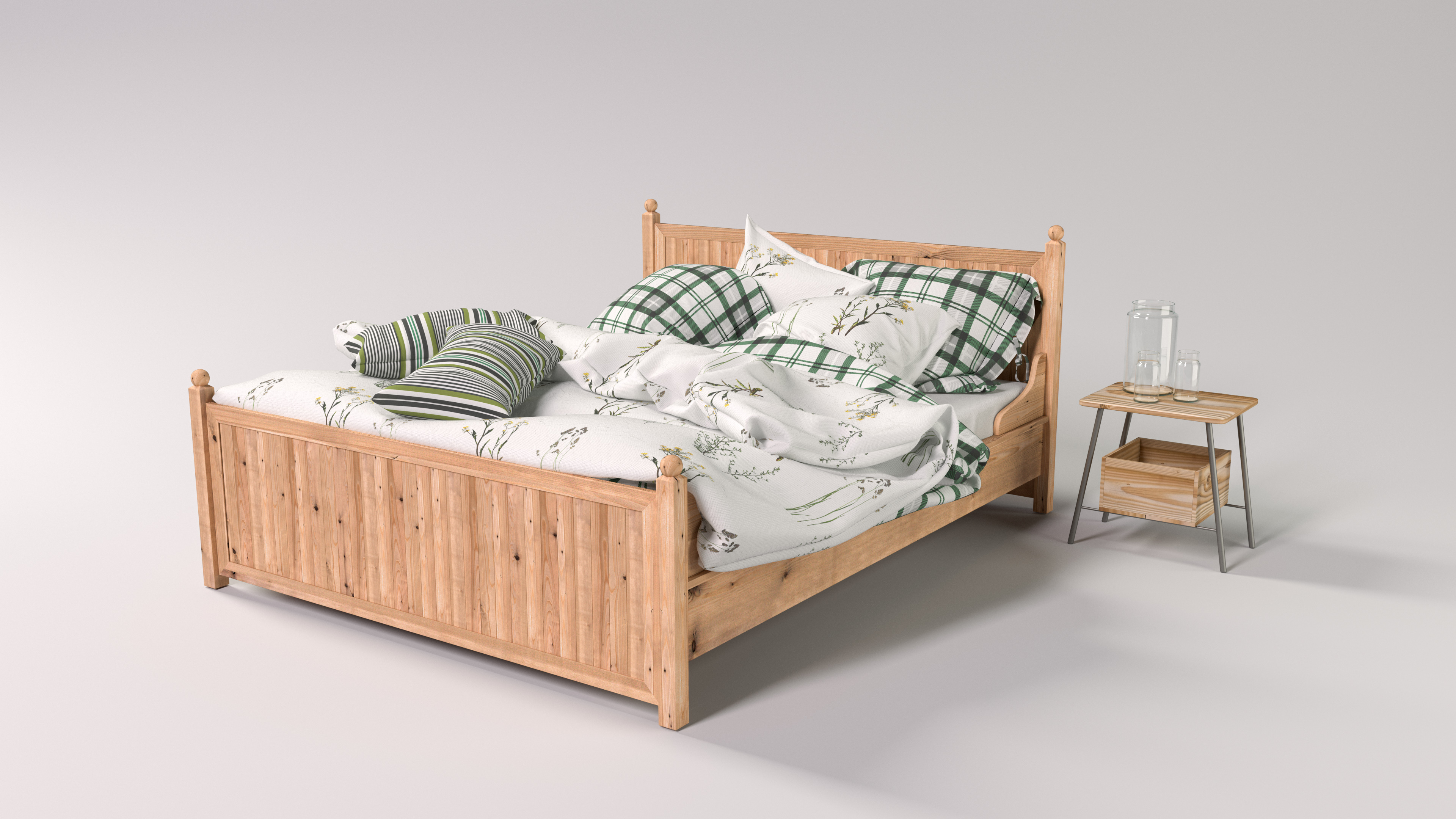
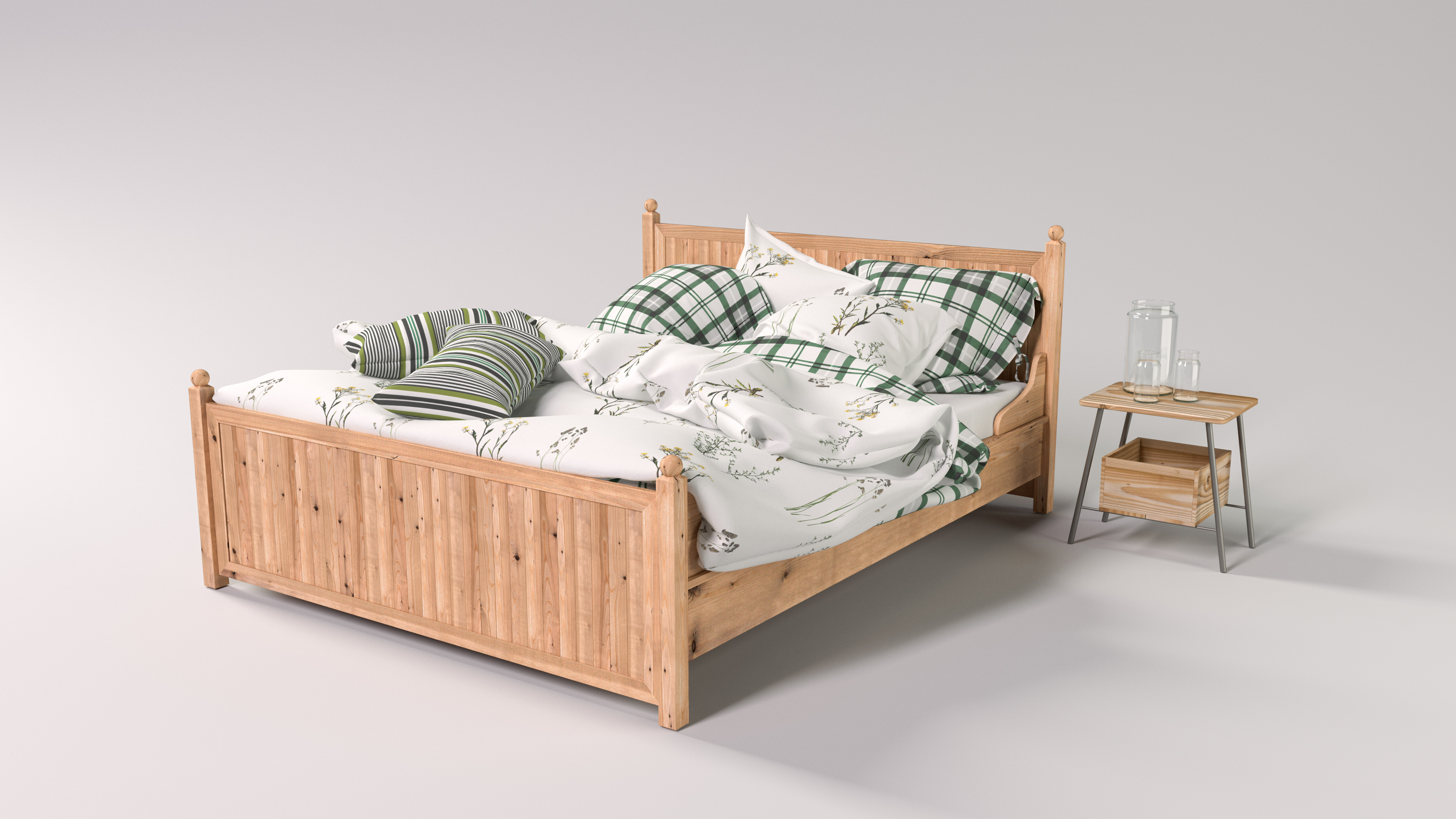
I recently implemented two techniques in Takua for solving the harsh shadow terminator problem; I implemented both the Disney Animation solution [Chiang et al. 2019] that we published at SIGGRAPH 2019, and the Sony Imageworks technique [Estevez et al. 2019] published in Ray Tracing Gems. We didn’t show too many comparisons between the two techniques (which I’ll refer to as the Chiang and Estevez approaches, respectively) in our SIGGRAPH 2019 presentation, and we didn’t show comparisons on any actual “real-world” scenes, so I thought I’d do a couple of my own renders using Takua as a bit of a mini-followup and share a handful of practical implementation tips. For a recap of the harsh shadow terminator problem, please see either the Estevez paper or the slides from the Chiang talk, which both do excellent jobs of describing the problem and why it happens in detail. Here’s a small scene that I made for this post, thrown together using some Evermotion assets that I had sitting around:

In this scene, all of the blankets and sheets and pillows on the bed use a fabric material that uses extremely high-frequency, high-resolution normal maps to achieve the fabric-y fiber-y look. Because of these high-frequency normal maps, the bedding is susceptible to the harsh shadow terminator problem. All of the bedding also has diffuse transmission and a very slight amount of high roughness specularity to emulate the look of a sheen lobe, making the material (and therefore this comparison) overall more interesting than just a single diffuse lobe.

Since the overall scene is pretty brightly lit and the bed is lit from all directions either by direct illumination from the window or bounce lighting from inside of the room, the shadow terminator problem is not as apparent in this scene; it’s still there, but it’s much more subtle than in the examples we showed in our talk. Below are some interactive comparisons between renders using Chiang 2019, Estevez 2019, and no shadow terminator fix; drag the slider left and right to compare:

If you would like to compare the 4K renders directly, they are located here: Chiang 2019, Estevez 2019, No Fix, No Normal Mapping. As mentioned above, due to this scene being brightly lit, differences between the two techniques and not having any harsh shadow terminator fix at all will be a bit more subtle. However, differences are still visible, especially in brighter areas of the blanket and white pillows. Note that in this scenario, the difference between Chiang 2019 and Estevez 2019 is fairly small, while the difference between using either shadow terminator fix and not having a fix is more apparent. Also note how both Chiang 2019 and Estevez 2019 produce results that come pretty close to matching the reference image with no normal mapping; this is good, since we would expect fix techniques to match the reference image more closely than not having a fix!

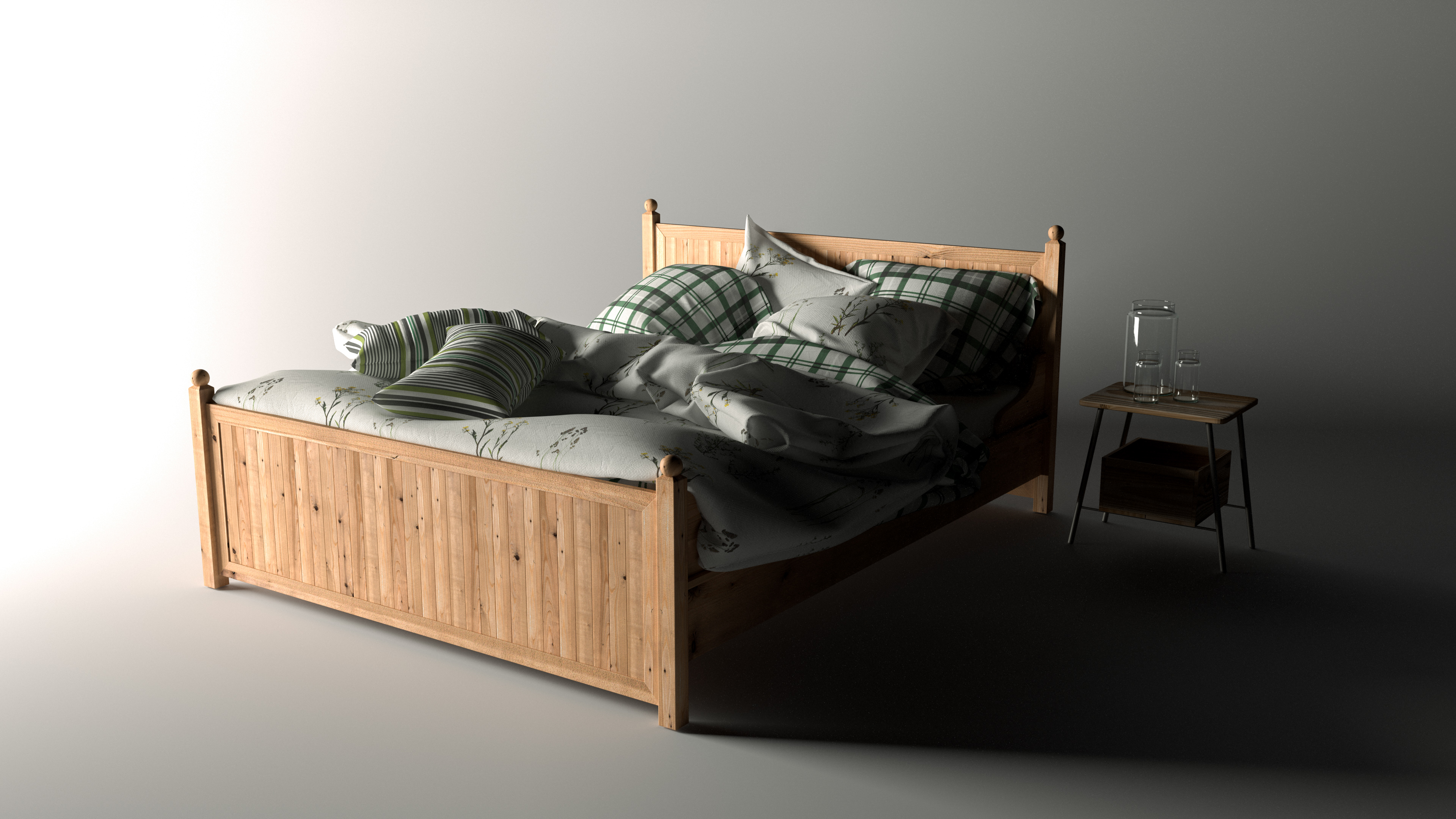
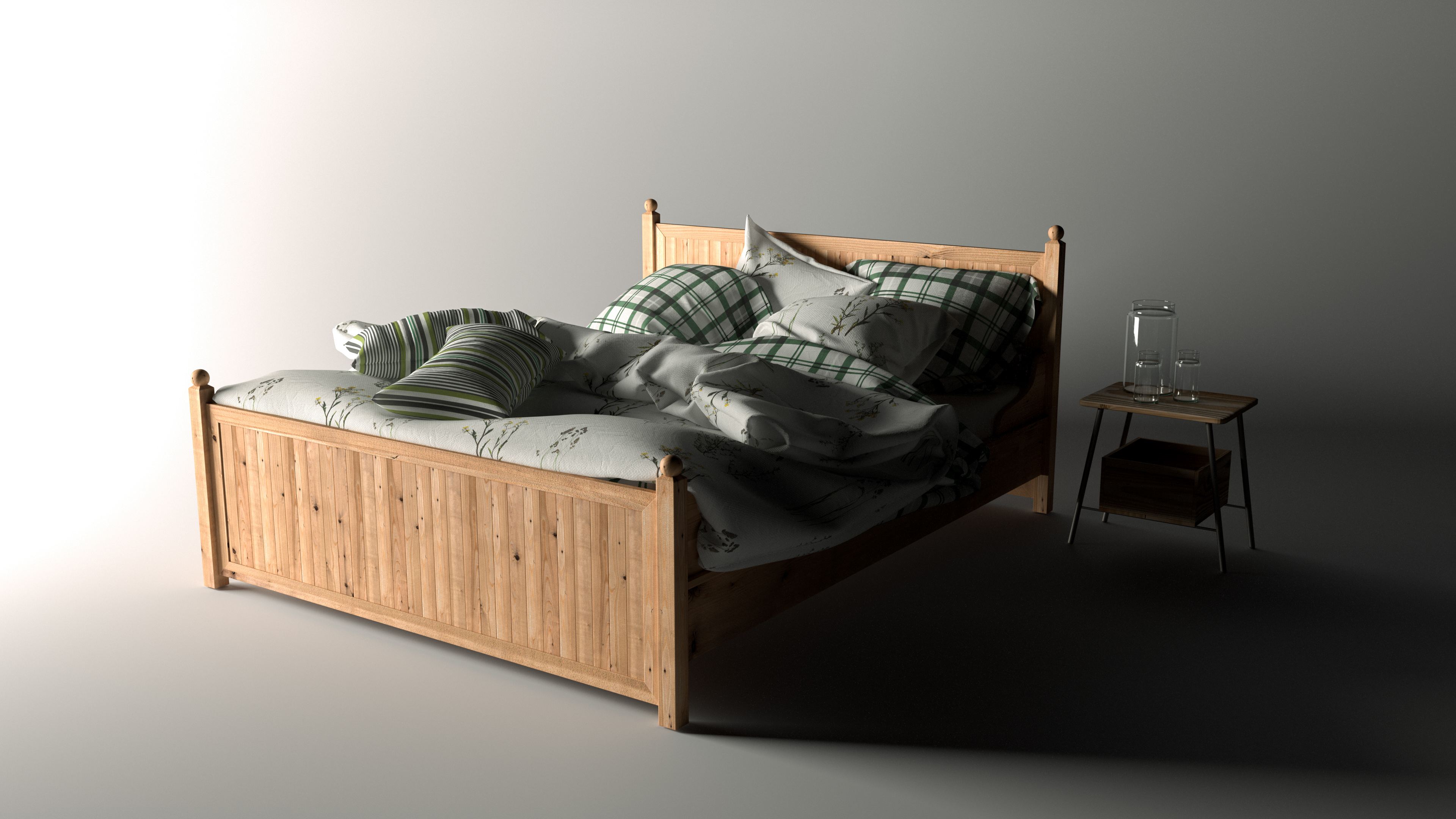
If we remove the bedroom set and put the bed onto more of a studio lighting setup with two area lights and a seamless grey backdrop, we can start seeing more prominent differences between the two techniques and between either technique and no fix. Seeing how everything plays out in this type of a lighting setup is useful, since this is the type of render that one often sees as part of a standard lookdev department’s workflow:

If you would like to compare the 4K renders directly for the studio lighting setup, they are located here: Chiang 2019, Estevez 2019, No Fix, No Normal Mapping. In this setup, we can now see differences between the four images much more clearly. Compared to the no normal mapping reference, the render with no fix produces considerably more darkening on silhouettes, and the harsh sudden transition from bright to shadowed areas is much more apparent. In the render with no fix, the bedding suddenly looks a lot less soft and starts to look a little more like a hard solid surface instead of like fabric.

Chiang 2019 and Estevez 2019 both restore more of the soft fabric look by softening out the harsh shadow terminator areas, but the differences between Chiang 2019 and Estevez 2019 become more apparent and interesting in this setting. Chiang 2019 produces an overall softer look that has shadow terminators that more closely match the reference with no normal mapping, but Chiang 2019 produces a slightly darker look overall compared to Estevez 2019. Estevez 2019 doesn’t match the reference’s shadow terminators quite as closely as Chiang 2019, but manages to preserve more of the overall energy. In Figure 5 in the Chiang 2019 paper, we explain where this difference comes from: for small shading normal deviations, Estevez 2019 produces less shadowing than our method, whereas for larger shading normal deviations, Estevez 2019 produces more shadowing than our method. As a result, Estevez 2019 generally produces a higher contrast look compared to Chiang 2019.

All of these differences are more apparent in a close-up crop of the full 4K render. Here are comparisons of the same studio lighting setup from above, but cropped in; pay close attention to slightly right of center of the image, where the white blanket overhangs the edge of the bed:

Of course, the scenario that makes the harsh shadow terminator problem the most apparent is when there is a single strong light source and we are viewing the scene from an angle from which we can see areas where the light hits surfaces at a glancing angle. These types of lighting setups are often used for checking silhouettes and backlighting and whatnot in modeling and lookdev turntable renders. In the comparisons below, the differences are most noticeable in the folds and on the shadowed sides of all of the bedding:

If you would like to compare the 4K renders directly for the single light source renders, they are located here: Chiang 2019, Estevez 2019, No Fix, No Normal Mapping. With a single light source, the differences between the four images are now very clear, since a single light setup produces strong contrast between the lit and shadowed parts of the image. The harsh shadow terminator problem is especially visible in the folds of the blanket, where we can see one side of the fold fully lit and one side of the fold in shadow (although because the bedding all has diffuse transmission, the harsh shadow terminator is still not as prevalent as it would be for a purely diffuse reflecting surface). Something else that is interesting is how the bedding with no shadow terminator fix overall appears slightly brighter than the bedding with no normal mapping; this is because the shading normals “bend” more light towards the light source. Chiang 2019 restores the overall brightness of the bedding back to something closer to the reference with no normal mapping but softens out more of the fine detail from the normal mapping, while Estevez 2019 preserves more of the fine details but has a brightness level closer to the render with no fix.

Just like in the studio lighting renders, differences become more apparent in close-up crops of the full 4K render. Here are some cropped in comparisons, this time centered more on the top of the bed than on the edge. In these crops, the glancing light angles make the shadow terminators more apparent in the folds of the blankets and such:

In the end, I don’t think either approach is better than the other, and from a physical basis there really isn’t a “right” answer since nothing about shading normals is physical to begin with; I think it’s up to a matter of personal preference and the requirements of the art direction on a given project. Our artists at Walt Disney Animation Studios generally prefer the look of Chiang 2019 because of the lighting setups they usually work with, but I know that other artists prefer the look of Estevez 2019 because they have different requirements to meet.

Fortunately, both Chiang 2019 and Estevez 2019 are both really easy to implement! Both techniques can be implemented in a handful of lines of code, and are easy to apply to any modern physically based shading model. We didn’t actually include source code in our SIGGRAPH talk, mostly because we figured that translating the math from our short paper into code should be very straightforward and thus, including source code that is basically a direct transcription of the math into C++ would almost be insulting to the intelligence of the reader. However, since then, I’ve gotten a surprising number of emails asking for source code, so here’s the math and the corresponding C++ code from my implementation in Takua Renderer. Let G’ be the additional shadow terminator term that we will multiply the Bsdf result with:

float calculateChiang2019ShadowTerminatorTerm(const vec3& outputDirection,
                                              const vec3& shadingNormal,
                                              const vec3& geometricNormal) {
    float NDotL = max(0.0f, dot(shadingNormal, outputDirection));
    float NGeomDotL = max(0.0f, dot(geometricNormal, outputDirection));
    float NGeomDotN = max(0.0f, dot(geometricNormal, shadingNormal));
    if (NDotL == 0.0f || NGeomDotL == 0.0f || NGeomDotN == 0.0f) {
        return 0.0f;
    } else {
        float G = NGeomDotL / (NDotL * NGeomDotN);
        if (G <= 1.0f) {
            float smoothTerm = -(G * G * G) + (G * G) + G; // smoothTerm is G' in the math
            return smoothTerm;
        }
    }
    return 1.0f;
}

That’s all there is to it! Source code for Estevez 2019 is provided as part of the Ray Tracing Gems Github repository, but for the sake of completeness, my implementation is included below. My implementation is just the sample implementation streamlined into a single function:

float calculateEstevez2019ShadowTerminatorTerm(const vec3& outputDirection,
                                               const vec3& shadingNormal,
                                               const vec3& geometricNormal) {
    float cos_d = min(abs(dot(geometricNormal, shadingNormal)), 1.0f);
    float tan2_d = (1.0f - cos_d * cos_d) / (cos_d * cos_d);
    float alpha2 = clamp(0.125f * tan2_d, 0.0f, 1.0f);

    float cos_i = max(abs(dot(geometricNormal, outputDirection)), 1e-6f);
    float tan2_i = (1.0f - cos_i * cos_i) / (cos_i * cos_i);
    float spi_shadow_term = 2.0f / (1.0f + sqrt(1.0f + alpha2 * tan2_i));
    return spi_shadow_term;
}

Finally, I have a handful of small implementation notes. First, to apply either Chiang 2019 or Estevez 2019 to your existing physically based shading model, just multiply the additional shadow terminator term with the contribution for each lobe that needs adjusting. Technically speaking G’ is an adjustment to the G shadowing term in a standard microfacet model, but multiplying there versus multiplying with the overall lobe contribution works out to be the same thing. If your Bsdf supports multiple shading normals for different specular lobes, you’ll need to calculate a separate shadow terminator term for each shading normal. Second, note that both Chiang 2019 and Estevez 2019 are described with respect to unidirectional path tracing from the camera. This frame of reference is very important; both techniques work specifically based on the outgoing direction being the direction towards a potential light source, meaning that this technique actually isn’t reciprocal by default. The Estevez 2019 paper found that the shadow terminator term can be made reciprocal by just applying the term to both incoming and outgoing directions, but they also found that this adjustment can make edges too dark. Instead, in order to make both techniques compatible with bidirectional path tracing integrators, I add in a check for whether the incoming or outgoing direction is pointed at a light, and feed the appropriate direction into the shadow terminator function. Doing this check is enough to make my bidirectional renders match my unidirectional ones; intuitively this approach is similar to the check one has to carry out when applying adjoint Bsdf adjustments [Veach 1996] for shading normals and refraction.

That’s pretty much it! If you want the details for how these two techniques are derived and why they work, I strongly encourage reading the Estevez 2019 chapter in Ray Tracing Gems and reading through both the short paper and the presentation slides / notes for the Chiang 2019 SIGGRAPH talk.

References

Matt Jen-Yuan Chiang, Yining Karl Li, and Brent Burley. 2019. Taming the Shadow Terminator. In ACM SIGGRAPH 2019 Talks. 71:1–71:2.

Alejandro Conty Estevez, Pascal Lecocq, and Clifford Stein. 2019. A Microfacet-Based Shadowing Function to Solve the Bump Terminator Problem. Ray Tracing Gems (2019), 149-158.

Eric Veach. 1996. Non-Symmetric Scattering in Light Transport Algorithms. In Rendering Techniques 1996 (Proceedings of the 7th Eurographics Workshop on Rendering). 82-91.

Errata

Thanks to Matt Pharr for noticing and pointing out a minor bug in the calculateChiang2019ShadowTerminatorTerm() implementation; the code has been updated with a fix.