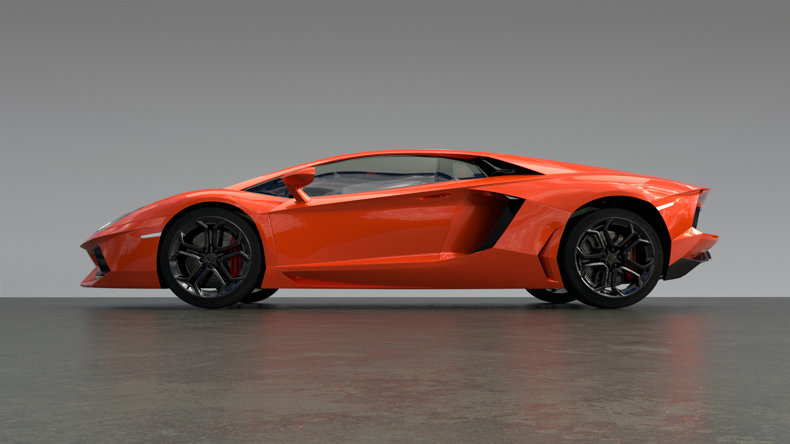
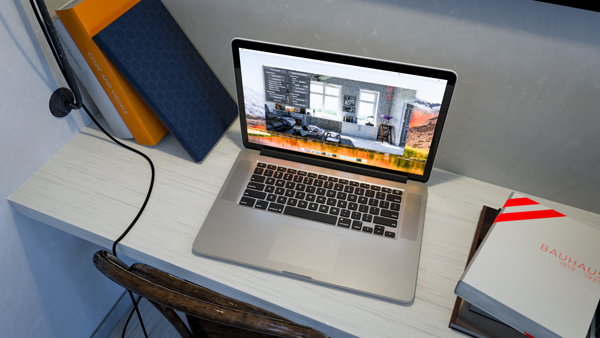
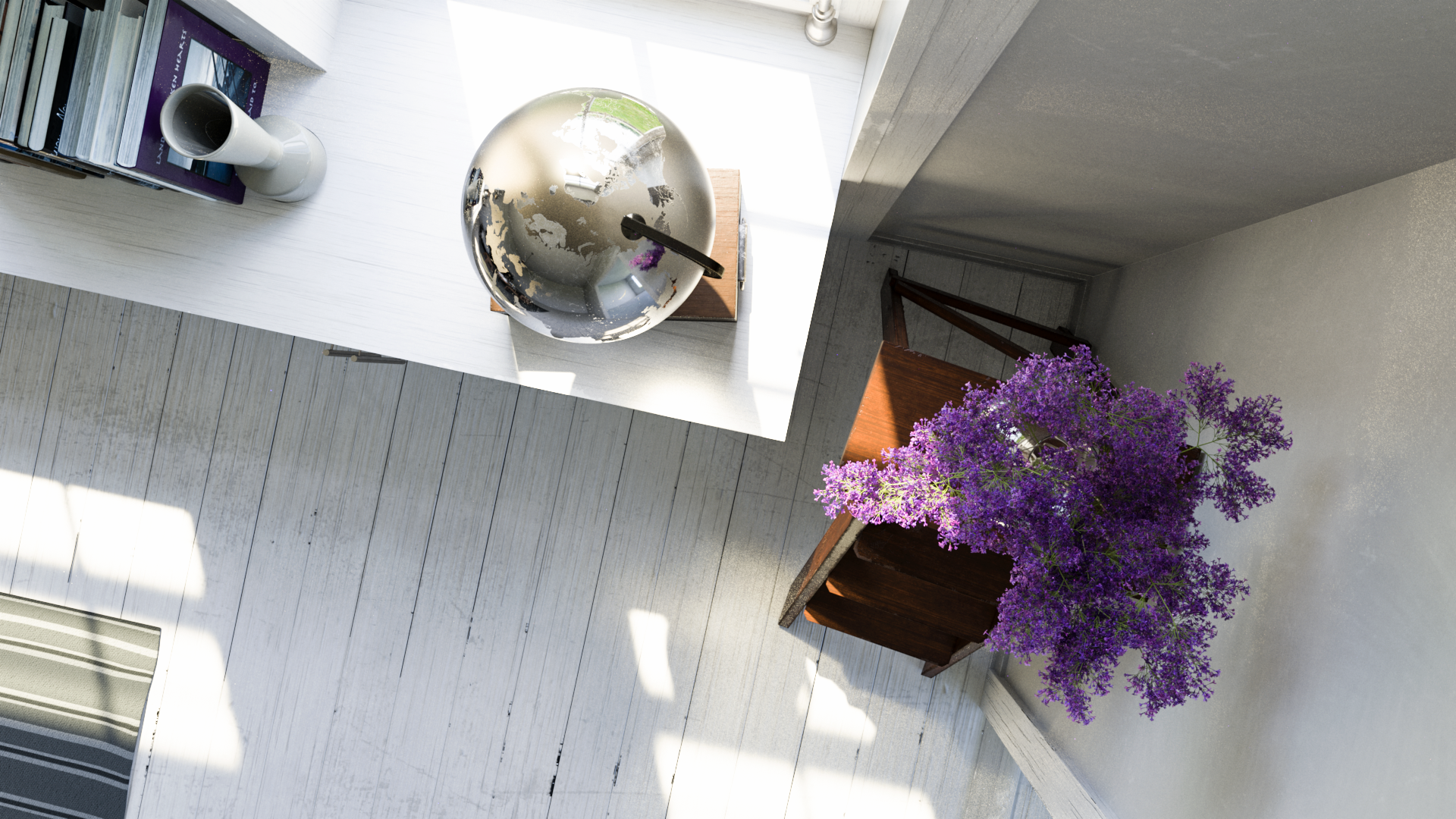
Almost three years ago, I rendered a small room interior scene to test an indoor, interior illumination scenario. Since then, a lot has changed in Takua, so I thought I’d revisit an interior illumination test with a much more complex, difficult scene. I don’t have much time to model stuff anymore these days, so instead I bought Evermotion’s Archinteriors Volume 48 collection, which is labeled as Scandinavian interior room scenes (I don’t know what’s particularly Scandinavian about these scenes, but that’s what the label said) and ported one of the scenes to Takua’s scene format. Instead of simply porting the scene as-is, I modified and added various things in the scene to make it feel a bit more customized. See if you can spot what they are:

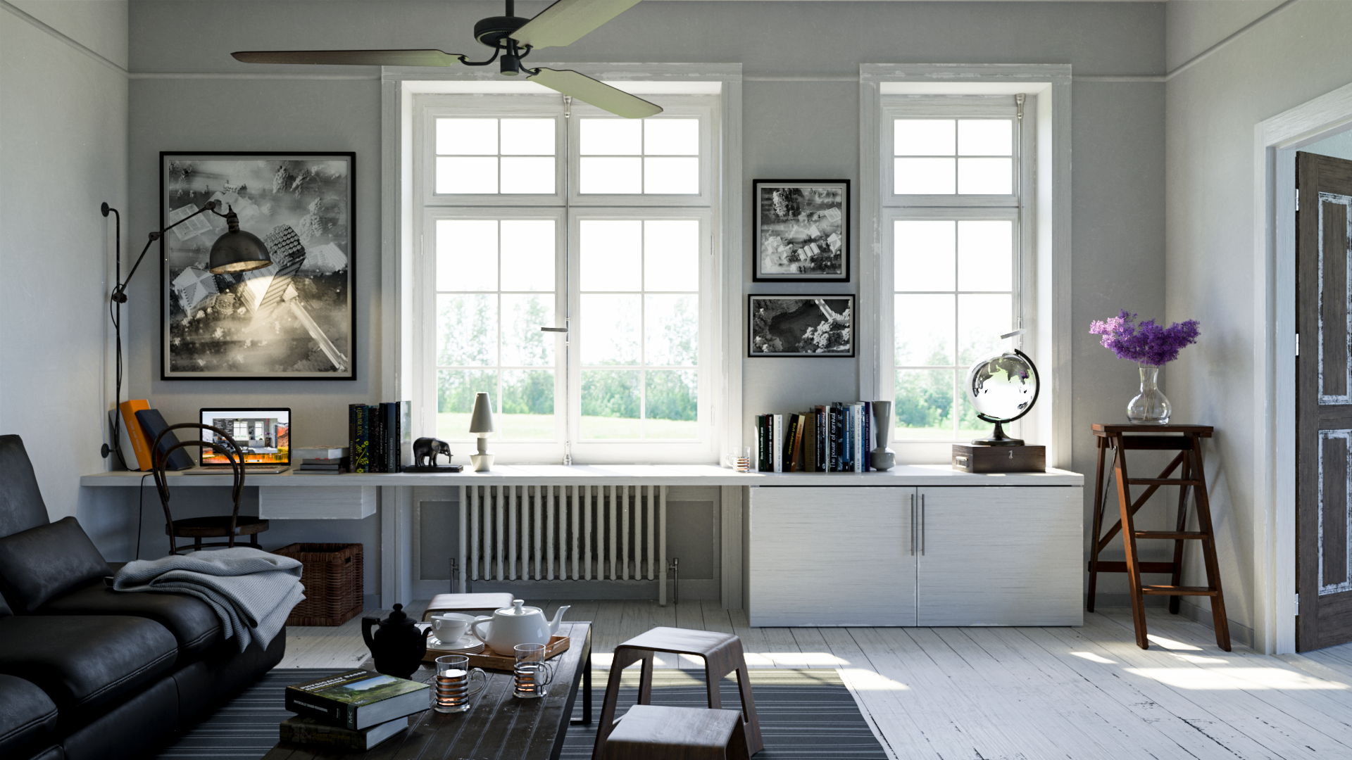
I had a lot of fun adding all of my customizations! I brought over some props from the old complex room scene, such as the purple flowers and vase, a few books, and Utah teapot tray, and also added a few new fun models, such as the MacBook Pro in the back and the copy of Physically Based Rendering 3rd Edition in the foreground. The black and white photos on the wall are crops of my Minecraft renders, and some of the books against the back wall have fun custom covers and titles. Even all of the elements that came with the original scene are re-shaded. The original scene came with Vray’s standard VrayMtl as the shader for everything; Takua’s base shader parameterization draws some influence from Vray, but also draws from the Disney Bsdf and Arnold’s AlShader and as a result has a parameterization that is sufficiently different that I wound up just re-shading everything instead of trying to write some conversion tool. For the most part I was able to re-use the textures that came with the scene to drive various shader parameters. The skydome is from the noncommercial version of VizPeople’s HDRi v1 collection.

Speaking of the skydome… the main source of illumination in this scene comes from the sun in the skydome, which presented a huge challenge for efficient light sampling. Takua has had domelight/environment map importance sampling using CDF inversion sampling for a long time now, which helps a lot, but the indoor nature of this scene still made sampling the sun difficult. Sampling the sun in an outdoor scene is fairly efficient since most rays will actually reach the sun, but in indoor scenes, importance sampling the sun becomes inefficient without taking occlusion into account since only rays that actually make it outdoors through windows can reach the sun. The best known method currently for handling domelight importance sampling through windows in an indoor scene is Portal Masked Environment Map Sampling (PMEMS) by Bitterli et al. I haven’t actually implemented PMEMS yet though, so the renders in this post all wound up requiring a huge number of samples per pixel to render; I intend on implementing PMEMS at some point in the near future.

Apart from the skydome, this scene also contains several other practical light sources, such as the lamp’s bulb, the MacBook Pro’s screen, and the MacBook Pro’s glowing Apple logo on the back of the screen (which isn’t even visible to camera, but is still enabled since it provides a tiny amount of light against the back wall!). In addition to choosing where on a single light to sample, choosing which light to sample is also an extremely important and difficult problem. Until this rendering this scene, I hadn’t really put any effort into efficiently selecting which light to sample. Most of my focus has been on the integration part of light transport, so Takua’s light selection has just been uniform random selection. Uniform random selection is terrible for scenes that contain multiple lights with highly varying emission between different lights, which is absolutely the case for this scene. Like any other importance sampling problem, the ideal solution is to send rays towards lights with a probability proportional to the amount of illumination we expect each light to contribute to each ray origin point.

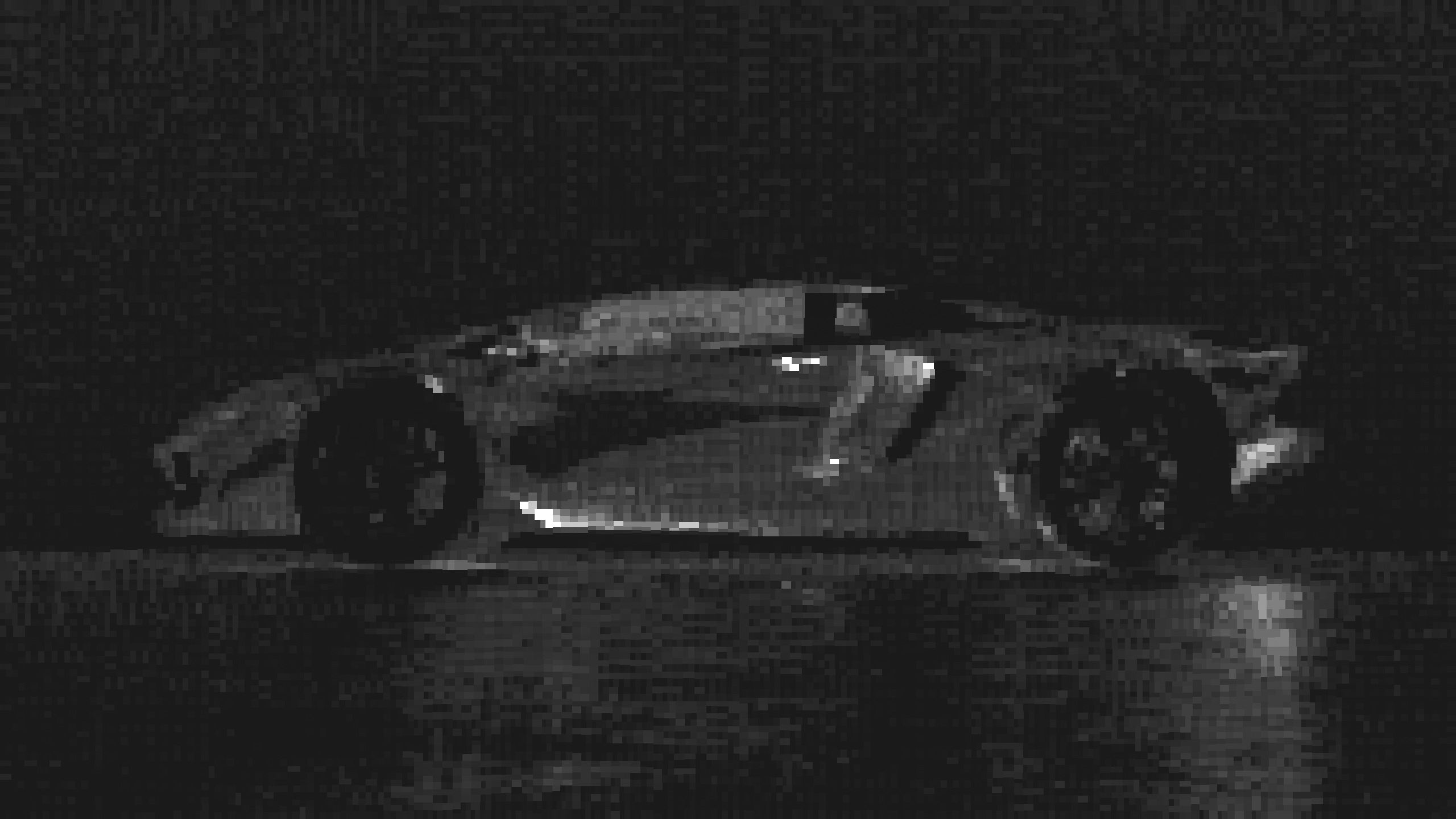
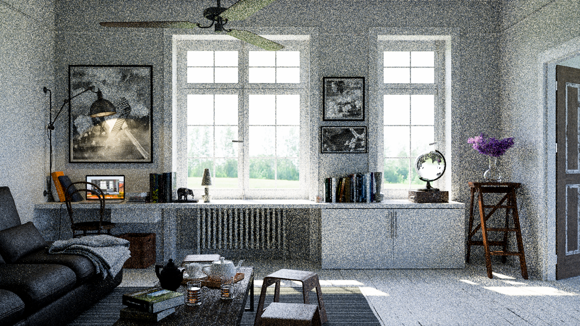
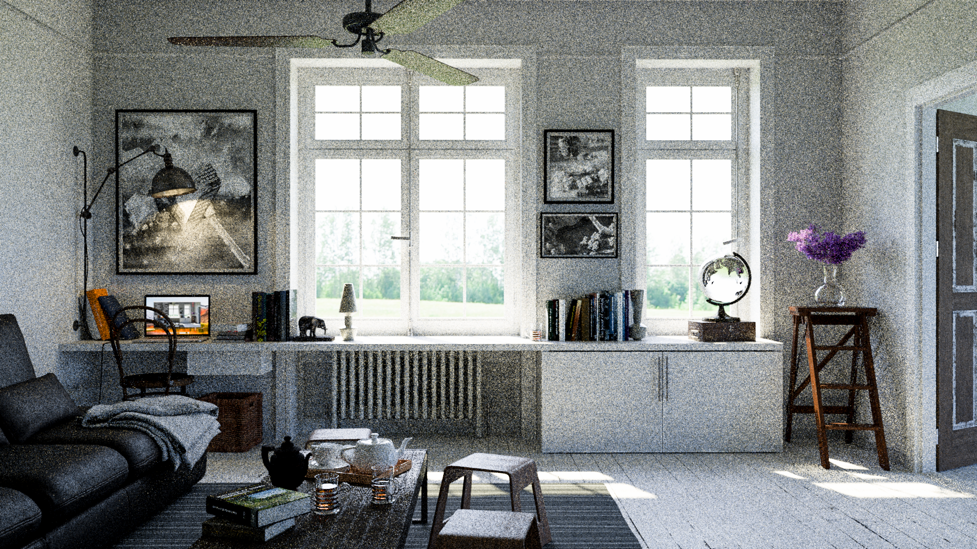
I implemented a light selection strategy where the probability of selecting each light is weighted by the total emitted power of each light; essentially this boils down to estimating the total emitted power of each light according to the light’s surface texture and emission function, building a CDF across all of the lights using the total emission estimates, and then using standard CDF inversion sampling to pick lights. This strategy works significantly better than uniform random selection and made a huge difference in render speed for this scene, as seen in Figures 2 through 4. Figure 2 uses uniform random light selection with 128 spp; note how the area lit by the wall-mounted lamp is well sampled, but the image overall is really noisy. Figure 3 uses power-weighted light selection with the same spp as Figure 2; the lamp area is more noisy than in Figure 2, but the render is less noisy overall. Notably, Figure 3 also took a third of the time compared to Figure 2 for the same sample count; this is because in this scene, sending rays towards the lamp is significantly more expensive due to heavier geometry than sending rays towards the sun, even when rays towards the sun get occluded by the walls. Figure 4 uses power-weighted light selection again, but is equal-time to Figure 2 instead of equal-spp; note the significant noise reduction:

However, power-weighted light selection still is not even close to being the most optimal technique possible; this technique completely ignores occlusion and distance, which are extremely important. Unfortunately, because occlusion and distance to each light varies for each point in space, creating a light selection strategy that takes occlusion and distance into account is extremely difficult and is a subject of continued research in the field. In Hyperion, we use a cache point system, which we described on page 97 of our SIGGRAPH 2017 Production Volume Rendering course notes. Other published research on the topic includes Practical Path Guiding for Efficient Light-Transport Simulation by Muller et al, On-line Learning of Parametric Mixture Models for Light Transport Simulation by Vorba et al, Product Importance Sampling for Light Transport Path Guiding by Herholz et al, Learning Light Transport the Reinforced Way by Dahm et al, and more. At some point in the future I’ll revisit this topic.

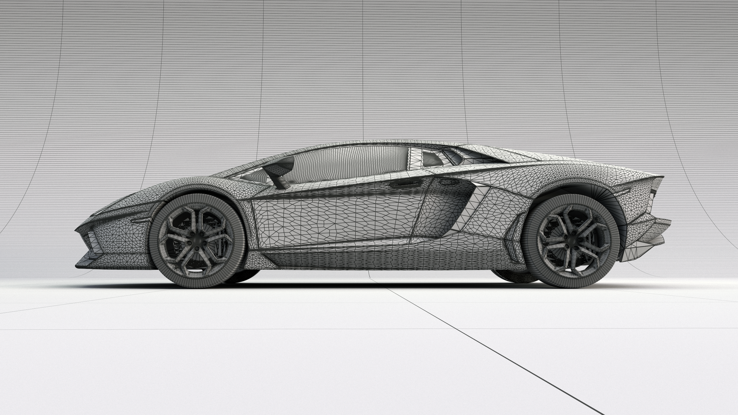
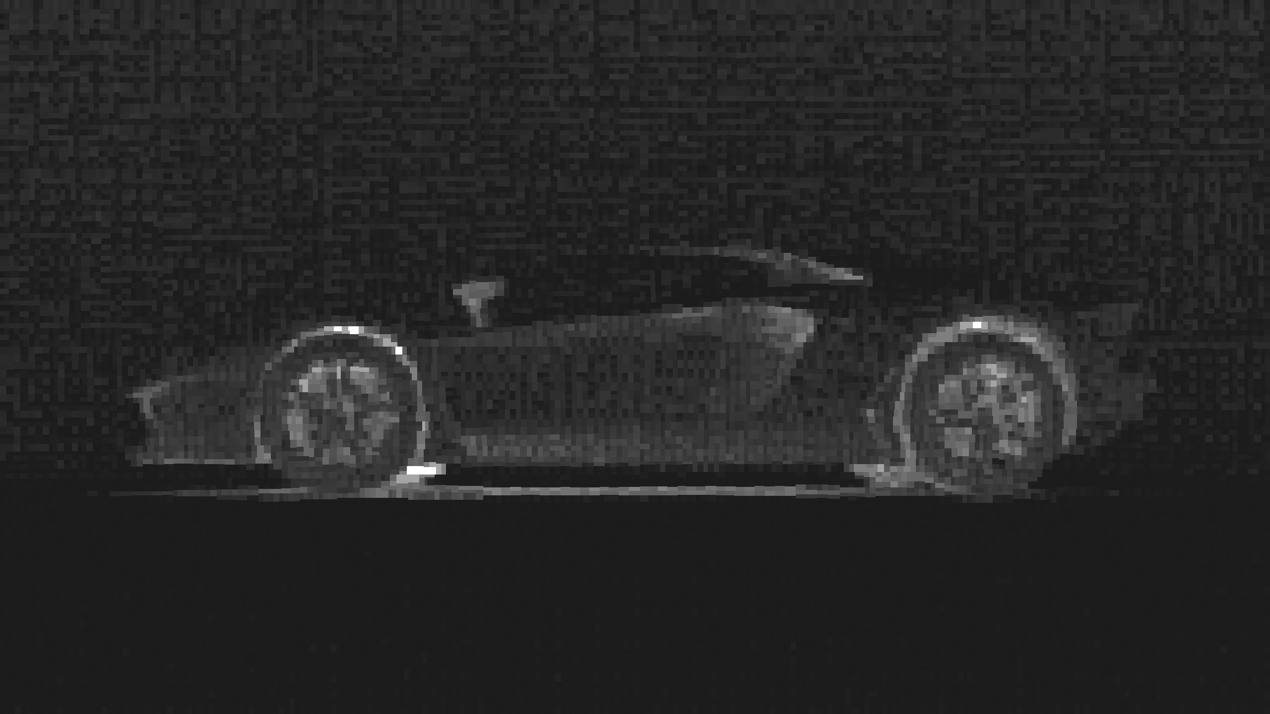
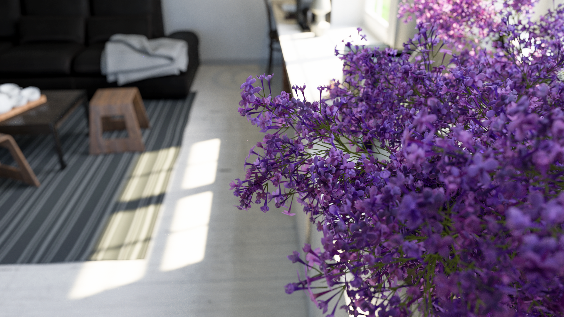
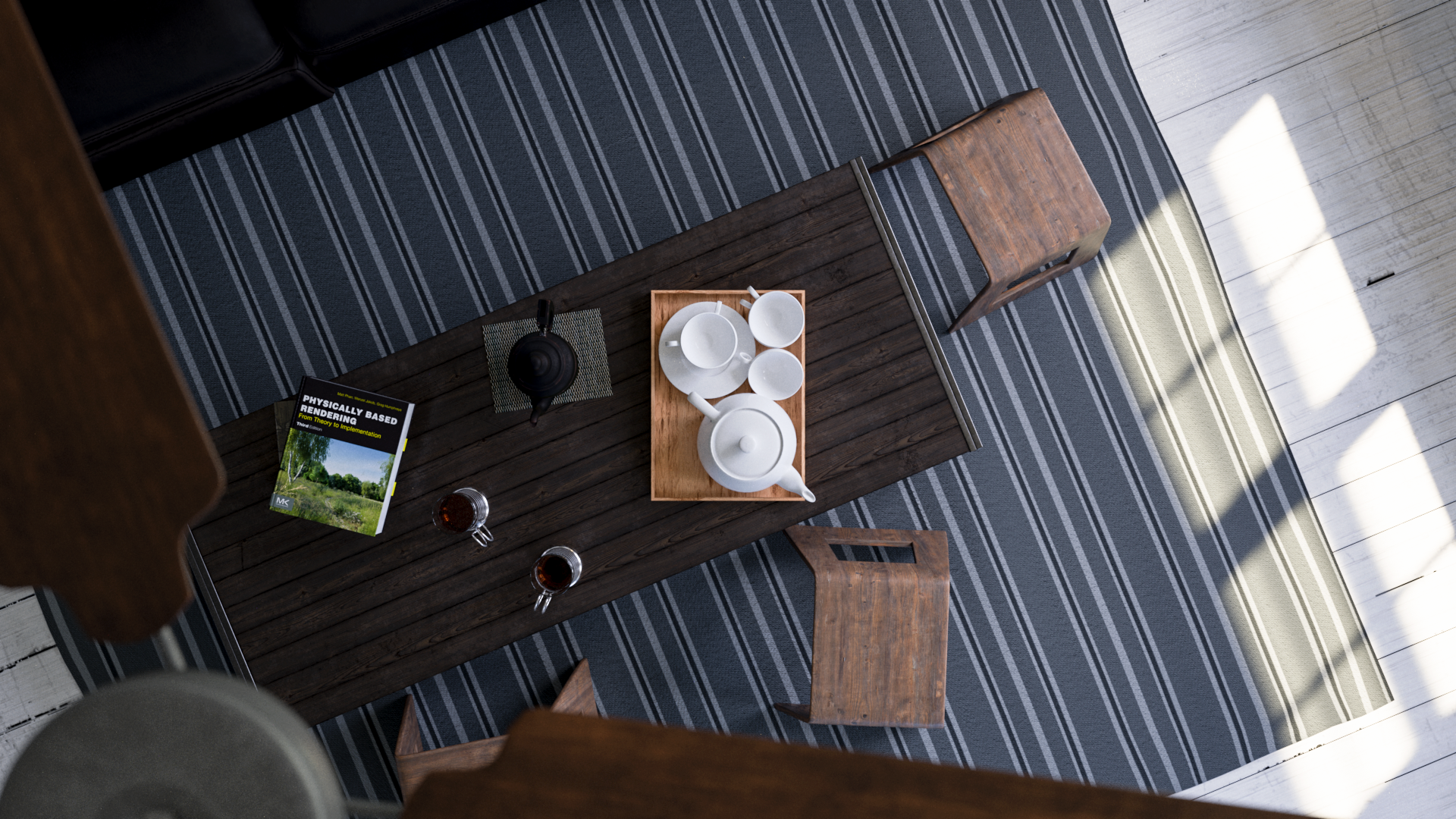
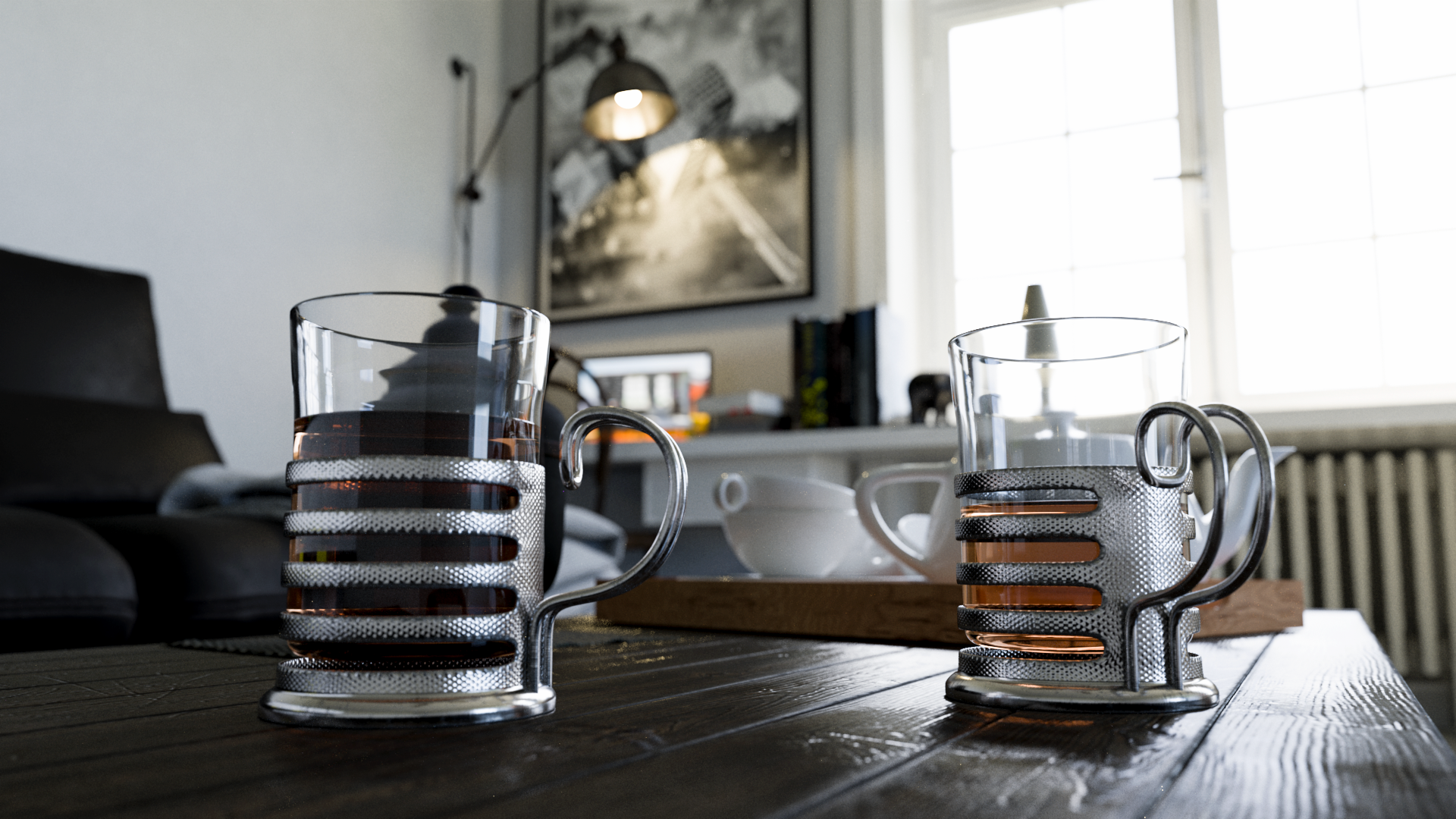
For a long time now, Takua has also had a simple interactive mode where the camera can be moved around in a non-shaded/non-lit view; I used this mode to interactively scout out some interesting and fun camera angles for some more renders. Being able to interactively scout in the same renderer used to final rendering is an extremely powerful tool; instead of guessing at depth of field settings and such, I was able to directly set and preview depth of field with immediate feedback. Unfortunately some of the renders below are noisier than I would like, due to the previously mentioned light sampling difficulties. All of the following images are rendered using Takua a0.8 with VCM:

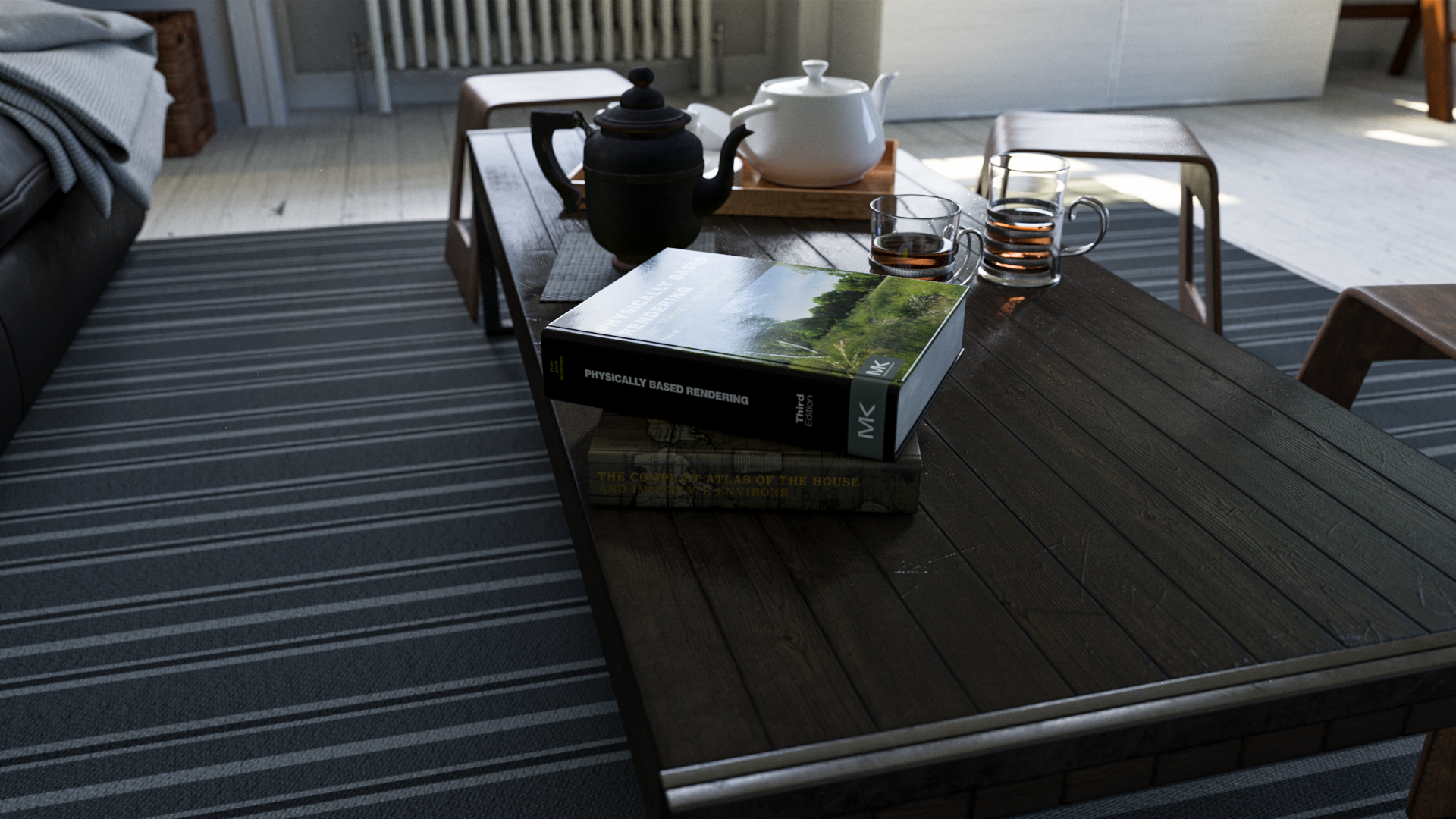
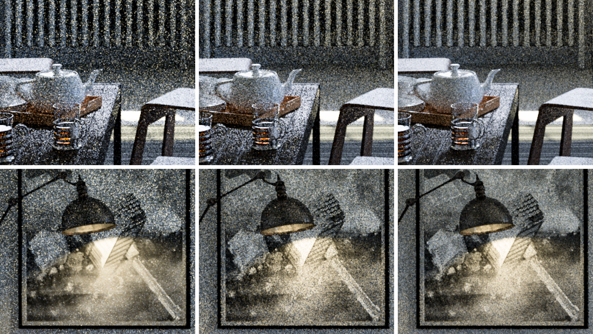
Beyond difficult light sampling, generally complex and difficult light transport with lots of subtle caustics also wound up presenting major challenges in this scene. For example, note the subtle caustics on the wall in the upper right hand part of Figure 10; those caustics are actually visibly not fully converged, even though the sample count across Figure 10 was in the thousands of spp! I intentionally did not use adaptive sampling in any of these renders; instead, I wanted to experiment with a common technique used in a lot of modern production renderers for noise reduction: in-render firefly clamping. My adaptive sampler is already capable of detecting firefly pixels and driving more samples at fireflies in the hopes of accelerating variance reduction on firefly pixels, but firefly clamping is a much more crude, biased, but nonetheless effective technique. The idea is to detect on each pixel spp if a returned sample is an outlier relative to all of the previously accumulated samples, and discard or clamp the sample if it in fact is an outlier. Picking what threshold to use for outlier detection is a very manual process; even Arnold provides a tuning max-value parameter for firefly clamping.

I wanted to be able to directly compare the render with and without firefly clamping, so I implemented firefly clamping on top of Takua’s AOV system. When enabled, firefly clamping mode produces two images for a single render: one output with firefly clamping enabled, and one with clamping disabled. I tried re-rendering Figure 10 using unidirectional pathtracing and a relatively low spp count to produce as many fireflies as I could, for a clearer comparison. For this test, I set the firefly threshold to be samples that are at least 250 times brighter than the estimated pixel value up to that sample.

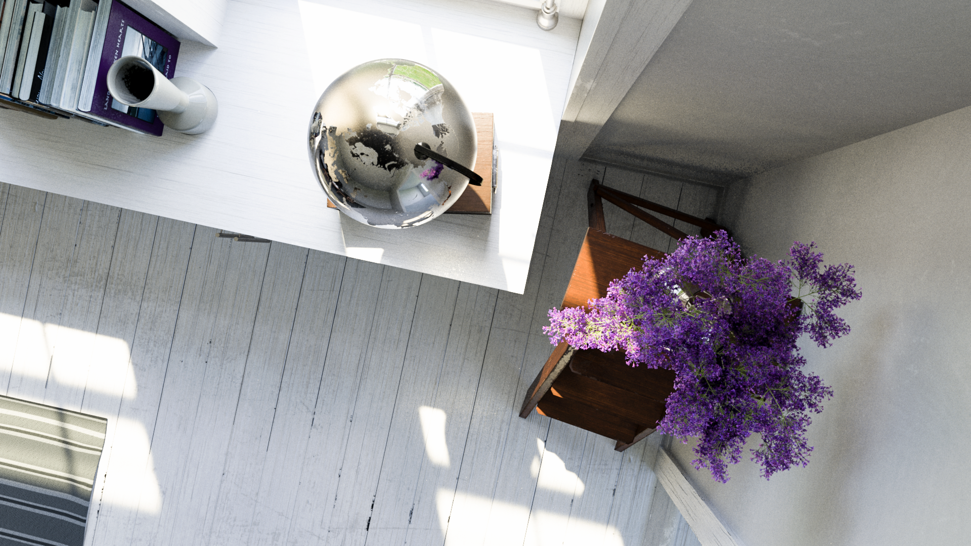
Note how Figure 13 appears to be completely firefly-free compared to Figure 12, and how Figure 13 doesn’t have visible caustic noise on the walls compared to Figure 10. However, notice how Figure 13 is also missing significant illumination in some areas, such as in the corner of the walls near the floor behind the wooden step ladder, or in the deepest parts of the purple flower bunch. Finding a threshold that eliminates all fireflies without loosing significant illumination in other areas is very difficult or, in some cases, impossible since some of these types of light transport essentially manifest as firefly-like high energy samples that only smooth out over time. For the final renders in Figure 1 and Figures 6 through 11, I wound up not actually using any firefly clamping. While biased noise-reduction techniques are a necessary evil in actual production, I expect that I’ll try to avoid relying on firefly clamping in the vast majority of what I do with Takua, since Takua is meant to just be a brute-force, hobby kind of thing anyway.

A long time ago, I made some posts that featured a cool Lamborghini Aventador model. Recently, I revisited that model and made some new renders using the current version of Takua, mostly just for fun. To me, one of the most important parts of writing a renderer has always been being able to actually use the renderer to make fun images. The last time I rendered this model was something like four years ago, and back then Takua was still in a very basic state; the renders in those old posts don’t even have any shading beyond 50% grey lambertian surfaces! The renders in this post utilize a lot of advanced features that I’ve added since then, such as a proper complex layered Bsdf and texturing system, advanced bidirectional light transport techniques, huge speed improvements to ray traversal, advanced motion blur and generalized time capabilities, and more. I’m way behind in writing up many of these features and capabilities, but in the meantime, I thought I’d post some for-fun rendering projects I’ve done with Takua.

All of the renders in this post are directly from Takua, with a basic white balance and conversion from HDR EXR to LDR PNG being the only post-processing steps. Each render took about half a day to render (except for the wireframe render, which was much faster) on a 12-core workstation at 2560x1440 resolution.

Shading the Aventador model was a fun, interesting exercise. I went for a orange-red paint scheme since, well, Lamborghinis are supposed to look outrageous and orange-red is a fairly exotic paint scheme (I suppose I could have picked green or yellow or something instead, but I like orange-red). I ended up making a triple-lobe shader with a metallic base, a dielectric lobe, and a clear-coat lobe on top of that. The base lobe uses a GGX microfacet metallic Brdf. Takua’s shading system implements a proper metallic Fresnel model for conductors, where the Fresnel model includes both a Nd component representing refractive index and a k component representing the extinction coefficient for when an electromagnetic wave propagates through a material. For conductors, the final Fresnel index of refraction for each wavelength of light is defined by a complex combination of Nd and k. For the base metallic lobe, most of the color wound up coming from the k component. The dielectric lobe is meant to simulate paint on top of a car’s metal body; the dielectric lobe is where most of the orange-red color comes from. The dielectric lobe is again a GGX microfacet Brdf, but with a dielectric Fresnel model, which has a much simpler index of refraction calculation than the metallic Fresnel model does. I should note that Takua’s current standard material implementation actually only supports a single primary specular lobe and an additional single clear-coat lobe, so for shaders authored with both a metallic and dielectric component, Takua takes a blend weight between the two components and for each shading evaluation stochastically selects between the two lobes according to the blend weight. The clear-coat layer on top has just a slightly amount of extinction to provide just a bit more of the final orange look, but is mostly just clear.

All of the window glass in the render is tinted slightly dark through extinction instead of through a fixed refraction color. Using proper extinction to tint glass is more realistic than using a fixed refraction color. Similarly, the red and yellow glass used in the head lights and tail lights are colored through extinction. The brake disks use an extremely high resolution bump map to get the brushed metal look. The branding and markings on the tire walls are done through a combination of bump mapping and adjusting the roughness of the microfacet Brdf; the tire treads are made using a high resolution normal map. There’s no displacement mapping at all, although in retrospect the tire treads probably should be displacement mapped if I want to put the camera closer to them. Also, I actually didn’t really shade the interior of the car much, since I knew I was going for exterior shots only.

Eventually I’ll get around to implementing a proper car paint Bsdf in Takua, but until then, the approach I took here seems to hold up reasonable well as long as the camera doesn’t get super close up to the car.

I lit the scene using two lights: an HDR skydome from HDRI-Skies, and a single long, thin rectangular area light above the car. The skydome provides the overall soft-ish lighting that illuminates the entire scene, and the rectangular area light provides the long, interesting highlights on the car body that help with bringing out the car’s shape.

For all of the renders in this post, I used my VCM integrator, since the scene contains a lot of subtle caustics and since the inside of the car is lit entirely through glass. I also wound up modifying my adaptive sampler; it’s still the same adaptive sampler that I’ve had for a few years now, but with an important extension. Instead of simply reducing the total number of paths per iteration as areas reach convergence, the adaptive sampler now keeps the number of paths the same and instead reallocates paths from completed pixels to high-variance pixels. The end result is that the adaptive sampler is now much more effective at eliminating fireflies and targeting caustics and other noisy areas. In the above render, some pixels wound up with as few as 512 samples, while a few particularly difficult pixels finished with as many as 20000 samples. Here is the adaptive sampling heatmap for Figure 1 above; brighter areas indicate more samples. Note how the adaptive sampler found a number of areas that we’d expect to be challenging, such as the interior through the car’s glass windows, and parts of the body with specular inter-reflections.

I recently implemented support for arbitrary camera shutter curves, so I thought doing a motion blurred render would be fun. After all, Lamborghinis are supposed to go fast! I animated the Lamborghini driving forward in Maya; the animation was very basic, with the main body just translating forward and the wheels both translating and rotating. Of course Takua has proper rotational motion blur. The motion blur here is effectively multi-segment motion blur; generating multi-segment motion blur from an animated sequence in Takua is very easy due to how Takua handles and understands time. I actually think that Takua’s concept of time is one of the most unique things in Takua; it’s very different from how every other renderer I’ve used and seen handles time. I intend to write more about this later. Instead of an instantaneous shutter, I used a custom cosine-based shutter curve that places many more time samples near the center of the shutter interval than towards the shutter open and close. Using a shutter shape like this wound up being important to getting the right look to the motion blur; even the car is moving extremely quickly, the overall form of the car is still clearly distinguishable and the front and back of the car appear more motion-blurred than the main body.

Since Takua has a procedural wireframe texture now, I also did a wireframe render. I mentioned my procedural wireframe texture in a previous post, but I didn’t write about how it actually works. For triangles and quads, the wireframe texture is simply based on the distance from the hitpoint to the nearest edge. If the distance to the nearest edge is smaller than some threshold, draw one color, otherwise, draw some other color. The nearest edge calculation can be done as follows (the variable names should be self-explanatory):

float calculateMinDistance(const Poly& p, const Intersection& hit) const {
    float md = std::numeric_limits<float>::infinity();
    const int verts = p.isQuad() ? 4 : 3;
    for (int i = 0; i < verts; i++) {
        const glm::vec3& cur = p[i].m_position;
        const glm::vec3& next = p[(i + 1) % verts].m_position;
        const glm::vec3 d1 = glm::normalize(next - cur);
        const glm::vec3 d2 = hit.m_point - cur;
        const float l = glm::length((cur + d1 * glm::dot(d1, d2) - hit.m_point));
        md = glm::min(md, l * l);
    }
    return md;
};

The topology of the meshes are pretty strange, since the car model came as a triangle mesh, which I then subdivided:

The material in the wireframe render only uses the lambertian diffuse lobe in Takua’s standard material; as such, the adaptive sampling heatmap for the wireframe render is interesting to compare to Figure 2. Overall the sample distribution is much more even, and areas where diffuse inter-reflections are present got more samples:

Takua’s shading model supports layering different materials through parameter blending, similar to how the Disney Brdf (and, at this point, most other shading systems) handles material layering. I wanted to make an even more outrageous looking version of the Aventador than the orange-red version, so I used the procedural wireframe texture as a layer mask to drive parameter blending between a black paint and a metallic gold paint:

After an amazing 2016, Walt Disney Animation Studios is having a bit of a break year this year. Disney Animation doesn’t have a feature film this year; instead, we made a half-hour featurette called Olaf’s Frozen Adventure, which will be released in front of Pixar’s Coco during Thanksgiving. I think this is the first time a Disney Animation short/featurette has accompanied a Pixar film. Olaf’s Frozen Adventure is a fun little holiday story set in the world of Frozen, and I had the privilege of getting to play a small role in making Olaf’s Frozen Adventure! I got an official credit as part of a handful of engineers that did some specific, interesting technology development for Olaf’s Frozen Adventure.

Olaf’s Frozen Adventure is really really funny; because Olaf is the main character, the entire story takes on much more of a self-aware, at times somewhat absurdist tone. The featurette also has a bunch of new songs- there are six new songs in total, which is somehow pretty close to the original film’s count of eight songs, but in a third of the runtime. Olaf’s Frozen Adventure was originally announced as a TV special, but the wider Walt Disney Company was so happy with the result that they decided to give Olaf’s Frozen Adventure a theatrical release instead!

Something I personally find fascinating about Olaf’s Frozen Adventure is comparing it visually with the original Frozen. Olaf’s Frozen Adventure is rendered entirely with Disney’s Hyperion Renderer, compared with Frozen, which was rendered using pre-RIS Renderman. While both films used our Disney BRDF [Burley 2012] and Ptex [Burley and Lacewell 2008], Olaf’s Frozen Adventure benefits from all of the improvements and advancements that have been made during Big Hero 6, Zootopia, and Moana. The original Frozen used dipole subsurface scattering, radiosity caching, and generally had fairly low geometric complexity relative to Hyperion-era films. In comparison, Olaf’s Frozen Adventure uses brute force subsurface scattering, uses path-traced global illumination, uses the full Disney BSDF (which is significantly extended from the Disney BRDF) [Burley 2015], uses our advanced fur/hair shader developed during Zootopia [Chiang et al. 2016], and has much greater geometric complexity. A great example of the greater geometric complexity is the knitted scarf sequence [Staub et al. 2018], where 2D animation was brought into Hyperion as a texture map to drive the colors on a knitted scarf that was modeled and rendered down to the fiber level. Some shots even utilize an extended version of the photon mapped caustics we developed during Moana; the photon mapped caustics system on Moana only supported distant lights as a photon source, but for Olaf’s Frozen Adventure, the photon mapping system was extended to support all of Hyperion’s existing light types as photon sources. These extensions to our photon mapping system is one of the things I worked on for Olaf’s Frozen Adventure, and was used for lighting the ice crystal tree that Elsa creates at the end of the film. Even the water in Arendelle Harbor looks way better than in Frozen, since the FX artists were able to make use of the incredible water systems developed for Moana [Palmer et al. 2017]. Many of these advancements are discussed in our SIGGRAPH 2017 Course Notes [Burley et al. 2017].

One of the huge advantages to working on an in-house production rendering team in a vertically integrated studio is being able to collaborate and partner closely with productions on executing long-term technical visions. Because of the show leadership’s confidence in our long-term development efforts targeted at later shows, the artists on Olaf’s Frozen Adventure were willing to take on and try out early versions of a number of new features in Hyperion that were originally targeted at later shows. Some of these “preview” features wound up making a big difference on Olaf’s Frozen Adventure, and lessons learned on Olaf’s Frozen Adventure were instrumental in making these features much more robust and complete on Ralph Breaks the Internet.

One major feature was brute force path-traced subsurface scattering; Peter Kutz, Matt Chiang, and Brent Burley had originally started development during Moana’s production on brute force path-traced subsurface scattering [Chiang 2016] as a replacement for Hyperion’s existing normalized diffusion based subsurface scattering [Burley 2015]. This feature wasn’t completed in time for use on Moana (although some initial testing was done using Moana assets), but was far enough along by Olaf’s Frozen Adventure was in production that artists started to experiment with it. If I remember correctly, the characters in Olaf’s Frozen Adventure are still using normalized diffusion, but path-traced subsurface wound up finding extensive use in rendering all of the snow in the show, since the additional detail that path-traced subsurface brings out helped highlight the small granular details in the snow. A lot of lessons learned from using path-traced subsurface scattering on the snow were then applied to making path-traced subsurface scattering more robust and easier to use and control. These experiences gave us the confidence to go ahead with full-scale deployment on Ralph Breaks the Internet, which uses path-traced subsurface scattering for everything including characters.

Another major development effort that found experimental use on Olaf’s Frozen Adventure were some large overhauls to Hyperion’s ray traversal system. During the production of Moana, we started running into problems with how large instance groups are structured in Hyperion. Moana’s island environments featured vast quantities of instanced vegetation geometry, and because of how the instancing was authored, Hyperion’s old strategy for grouping instances in the top-level BVH wound up producing heavily overlapping BVH leaves, which in extreme cases could severely degrade traversal performance. On Moana, the solution to this problem was to change how instances were authored upstream in the pipeline, but the way that the renderer wanted instances organized was fairly different from how artists and our pipeline like to think about instances, which made authoring more difficult. This problem motivated Peter Kutz and I to develop a new traversal system that would be less sensitive to how instance groups were authored; the system we came up with allows Hyperion to internally break up top-level BVH nodes with large overlapping bounds into smaller, tighter subbounds based on the topology of the lower-level BVHs. It turns out this system is conceptually essentially identical to BVH rebraiding [Benthin et al. 2017], but we developed and deployed this system independently before Benthin 2017 was published. As part of this effort, we also wound up revisiting Hyperion’s original cone-based packet traversal strategy [Eisenacher et al. 2013] and, motivated by extensive testing and statistical performance analysis, developed a new, simpler, higher performance multithreading strategy for handling Hyperion’s ultra-wide batched ray traversal. Olaf’s Frozen Adventure has a sequence where Olaf and Sven are being pulled down a mountainside through a forest by a burning sled; the enormous scale of the groundplane and large quantities of instanced trees proved to be challenging for Hyperion’s old traversal system. We were able to partner with the artists to deploy a mid-development prototype of our new traversal system on this sequence, and were able to cut traversal times by up to close to an order of magnitude in some cases. As a result, the artists were able to render this sequence with reasonable render times, and we were able to field-test the new traversal system prior to studio-wide deployment and iron out various kinks that were found along the way.

The last major mid-development Hyperion feature that saw early experimental use on Olaf’s Frozen Adventure was our new, next-generation spectral and decomposition tracking [Kutz et al. 2017] based null-collision volume rendering system, which was written with the intention of eventually completely replacing Hyperion’s existing residual ratio tracking [Novák 2014] based volume rendering system [Fong 2017]. Artists on Olaf’s Frozen Adventure ran into some difficulties with rendering loose, fluffy white snow, where the bright white appearance is the result of high-order scattering requiring large numbers of bounces. We realized that this problem is essentially identical to the problem of rendering white puffy clouds, which also have an appearance dominated by energy from high-order scattering. Since null-collision volume integration is specifically very efficient at handling high-order scattering, we gave the artists an early prototype version of Hyperion’s new volume rendering system to experiment with rendering loose fluffy snow as a volume. The initial results looked great; I’m not sure if this approach wound up being used in the final film, but this experiment gave both us and the artists a lot of confidence in the new volume rendering system and provided valuable feedback.

As usual with Disney Animation projects I get to work on, here are some stills in no particular order, from the film. Even though Olaf’s Frozen Adventure was originally meant for TV, the whole studio still put the same level of effort into it that goes into full theatrical features, and I think it shows!

Here is a credits frame with my name! I wasn’t actually expecting to get a credit on Olaf’s Frozen Adventure, but because I had spent a lot of time supporting the show and working with artists on deploying experimental Hyperion features to solve particularly difficult shots, the show decided to give me a credit! I was very pleasantly surprised by that; my teammate Matt Chiang got a credit as well for similar reasons.

All images in this post are courtesy of and the property of Walt Disney Animation Studios.

References

Carsten Benthin, Sven Woop, Ingo Wald, and Attila T. Áfra. 2017. Improved Two-Level BVHs using Partial Re-Braiding. In Proc. of High Performance Graphics (HPG 2017). Article 7.

Brent Burley. 2012. Physically Based Shading at Disney. In ACM SIGGRAPH 2012 Course Notes: Practical Physically-Based Shading in Film and Game Production.

Brent Burley. 2015. Extending the Disney BRDF to a BSDF with Integrated Subsurface Scattering. In ACM SIGGRAPH 2015 Course Notes: Physically Based Shading in Theory and Practice.

Brent Burley, David Adler, Matt Jen-Yuan Chiang, Ralf Habel, Patrick Kelly, Peter Kutz, Yining Karl Li, and Daniel Teece. 2017. Recent Advances in Disney’s Hyperion Renderer. In ACM SIGGRAPH 2017 Course Notes: Path Tracing in Production Part 1

Brent Burley and Dylan Lacewell. 2008. Ptex: Per-face Texture Mapping for Production Rendering. Computer Graphics Forum (Proc. of Eurographics Symposium on Rendering) 27, 4 (Jun. 2008), 1155-1164.

Matt Jen-Yuan Chiang, Benedikt Bitterli, Chuck Tappan, and Brent Burley. 2016. A Practical and Controllable Hair and Fur Model for Production Path Tracing. Computer Graphics Forum (Proc. of Eurographics) 35, 2 (May 2016), 275-283.

Matt Jen-Yuan Chiang, Peter Kutz, and Brent Burley. 2016. Practical and Controllable Subsurface Scattering for Production Path Tracing. In ACM SIGGRAPH 2016 Talks. Article 49.

Christian Eisenacher, Gregory Nichols, Andrew Selle, and Brent Burley. 2013. Sorted Deferred Shading for Production Path Tracing. Computer Graphics Forum (Proc. of Eurographics Symposium on Rendering) 32, 4 (Jul. 2013), 125-132.

Julian Fong, Magnus Wrenninge, Christopher Kulla, and Ralf Habel. 2017. Production Volume Rendering. In ACM SIGGRAPH 2017 Courses. Article 2.

Peter Kutz, Ralf Habel, Yining Karl Li, and Jan Novák. 2017. Spectral and Decomposition Tracking for Rendering Heterogeneous Volumes. ACM Transactions on Graphics (Proc. of SIGGRAPH) 36, 4 (Aug. 2017), Article 111.

Jan Novák, Andrew Selle and Wojciech Jarosz. 2014. Residual Ratio Tracking for Estimating Attenuation in Participating Media. ACM Transactions on Graphics (Proc. of SIGGRAPH Asia) 33, 6 (Nov. 2014), Article 179.

Sean Palmer, Jonathan Garcia, Sara Drakeley, Patrick Kelly, and Ralf Habel. 2017. The Ocean and Water Pipeline of Disney’s Moana. In ACM SIGGRAPH 2017 Talks. Article 29.

Josh Staub, Alessandro Jacomini, Dan Lund. 2018. The Handiwork Behind “Olaf’s Frozen Adventure”. In ACM SIGGRAPH 2018 Talks. Article 26.

This year at SIGGRAPH 2017, Luca Fascione and Johannes Hanika from Weta Digital organized a Path Tracing in Production course. The course was split into two halves: a first half about production renderers, and a second half about using production renderers to make movies. Brent Burley presented our recent work on Disney’s Hyperion Renderer as part of the first half of the course. To support Brent’s section of the course, the entire Hyperion team worked together to put together some course notes describing recent work in Hyperion done for Zootopia, Moana, and upcoming films.

Here is the abstract for the course notes:

Path tracing at Walt Disney Animation Studios began with the Hyperion renderer, first used in production on Big Hero 6. Hyperion is a custom, modern path tracer using a unique architecture designed to efficiently handle complexity, while also providing artistic controllability and efficiency. The concept of physically based shading at Disney Animation predates the Hyperion renderer. Our history with physically based shading significantly influenced the development of Hyperion, and since then, the development of Hyperion has in turn influenced our philosophy towards physically based shading.

The course notes and related materials can be found at:

• Official Course Resources Page (Full course notes and supplemental materials)
• Project Page (Author’s Version)
• Official Print Version (ACM Library)

The course wasn’t recorded due to proprietary content from various studios, but the overall course notes for the entire course cover everything that was presented. The major theme of our part of the course notes (and Brent’s presentation) is replacing multiple scattering approximations with accurate brute-force path-traced solutions. Interestingly, the main motivator for this move is primarily a desire for better, more predictable and intuitive controls for artists, as opposed to simply just wanting better visual quality. In the course notes, we specifically discuss fur/hair, path-traced subsurface scattering, and volume rendering.

The Hyperion team also had two other presentations at SIGGRAPH 2017:

• Ralf Habel presented several sections of the “Production Volume Rendering”” course, which was jointly put together by Julian Fong and Magnus Wrenninge from Pixar Animation Studios, Christophe Kulla from Sony Imageworks, and Ralf Habel from Walt Disney Animation Studios.
• Peter Kutz presented our “Spectral and Decomposition Tracking for Rendering Heterogeneous Volumes” technical paper in the “Rendering Volumes” papers session.