Two standard features that every modern production renderer supports are subdivision surfaces and some form of displacement mapping. As we’ll discuss a bit later in this post, these two features are usually very closely linked to each other in both usage and implementation. Subdivision and displacement are crucial tools for representing detail in computer graphics; from both a technical and authorship point of view, being able to represent more detail than is actually present in a mesh is advantageous. Applying detail at runtime allows for geometry to take up less disk space and memory than would be required if all detail was baked into the geometry, and artists often like the ability to separate broad features from high frequency detail.

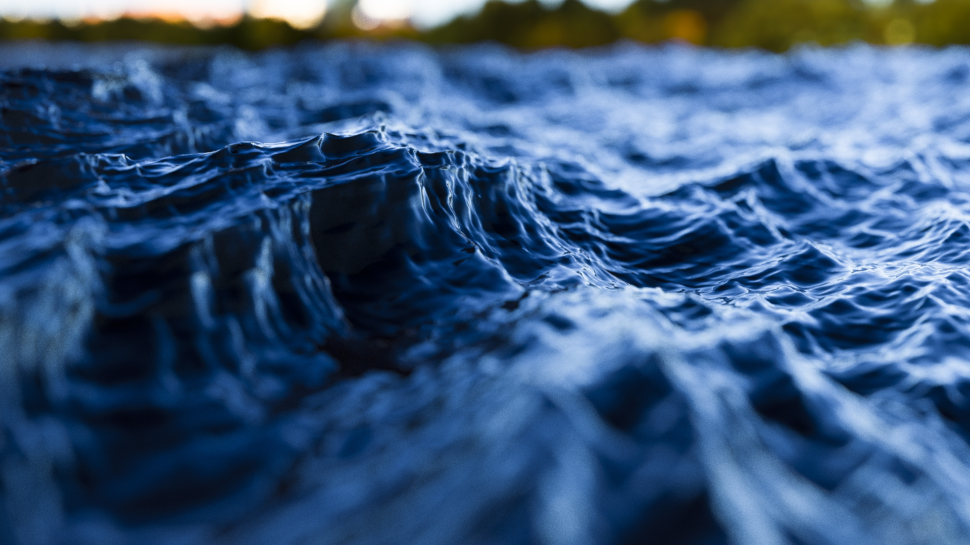
I recently added support for subdivision surfaces and for both scalar and vector displacement to Takua; Figure 1 shows an ocean wave was rendered using vector displacement in Takua. The ocean surface is entirely displaced from just a single plane!

Both subdivision and displacement originally came from the world of rasterization rendering, where on-the-fly geometry generation was historically both easier to implement and more practical/plausible to use. In rasterization, geometry is streamed to through the renderer and drawn to screen, so each individual piece of geometry could be subdivided, tessellated, displaced, splatted to the framebuffer, and then discarded to free up memory. Old REYES Renderman was famously efficient at rendering subdivision surfaces and displacement surfaces for precisely this reason. However, in naive ray tracing, rays can intersect geometry at any moment in any order. Subdividing and displacing geometry on the fly for each ray and then discarding the geometry is insanely expensive compared to processing geometry once across an entire framebuffer. The simplest solution to this problem is to just subdivide and displace everything up front and keep it all around in memory during ray tracing. Historically though, just caching everything was never a practical solution since computers simply didn’t have enough memory to keep that much data around. As a result, past research work put significant effort into more intelligent ray tracing architectures that made on-the-fly subdivision/displacement affordable again; notable advancements include geometry caching for ray tracing [Pharr and Hanrahan 1996], direct ray tracing of displacement mapped triangles [Smits et al. 2000], reordered ray tracing [Hanika et al. 2010], and GPU ray traced vector displacement [Harada 2015].

In the past five years or so though, the story on ray traced displacement has changed. We now have machines with gobs and gobs of memory (at a number of studios, renderfarm nodes with 256 GB of memory or more is not unusual anymore). As a result, ray traced renderers don’t need to be nearly as clever anymore about managing displaced geometry; a combination of camera-adaptive tessellation and a simple geometry cache with a least-recently-used eviction strategy is often enough to make ray traced displacement practical. Heavy displacement is now common in the workflows for a number of production pathtracers, including Arnold, Renderman/RIS, Vray, Corona, Hyperion, Manuka, etc. With the above in mind, I tried to implement subdivision and displacement in Takua as simply as I possibly could.

Takua doesn’t have any concept of an eviction strategy for cached tessellated geometry; the hope is to just fit in memory and be as efficient as possible with what memory is available. Admittedly, since Takua is just my hobby renderer instead of a fully in-use production renderer, and I have personal machines with 48 GB of memory, I didn’t think particularly hard about cases where things don’t fit in memory. Instead of tessellating on-the-fly per ray or anything like that, I simply pre-subdivide and pre-displace everything upfront during the initial scene load. Meshes are loaded, subdivided, and displaced in parallel with each other. If Takua discovers that all of the subdivided and displaced geometry isn’t going to fit in the allocated memory budget, the renderer simply quits.

I should note that Takua’s scene format distinguishes between a mesh and a geom; a mesh is the raw vertex/face/primvar data that makes up a surface, while a geom is an object containing a reference to a mesh along with transformation matrices, shader bindings, and so on and so forth. This separation between the mesh data and the geometric object allows for some useful features in the subdivision/displacement system. Takua’s scene file format allows for binding subdivision and displacement modifiers either on the shader level, or per each geom. Bindings at the geom level override bindings on the shader level, which is useful for authoring since a whole bunch of objects can share the same shader but then have individual specializations for different subdivision rates and different displacement maps and displacement settings. During scene loading, Takua analyzes what subdivisions/displacements are required for which meshes by which geoms, and then de-duplicates and aggregates any cases where different geoms want the same subdivision/displacement for the same mesh. This de-duplication even works for instances (I should write a separate post about Takua’s approach to instancing someday…).

Once Takua has put together a list of all meshes that require subdivision, meshes are subdivided in parallel. For Catmull-Clark subdivision [Catmull and Clark 1978], I rely on OpenSubdiv for calculating subdivision stencil tables [Halstead et al. 1993] for feature adaptive subdivision [Nießner et al. 2012], evaluating the stencils, and final tessellation. As far as I can tell, stencil calculation in OpenSubdiv is single threaded, so it can get fairly slow on really heavy meshes. Stencil evaluation and final tessellation is super fast though, since OpenSubdiv provides a number of parallel evaluators that can run using a variety of backends ranging from TBB on the CPU to CUDA or OpenGL compute shaders on the GPU. Takua currently relies on OpenSubdiv’s TBB evaluator. One really neat thing about the stencil implementation in OpenSubdiv is that the stencil calculation is dependent on only the topology of the mesh and not individual primvars, so a single stencil calculation can then be reused multiple times to interpolate many different primvars, such as positions, normals, uvs, and more. Currently Takua doesn’t support creases; I’m planning on adding crease support later.

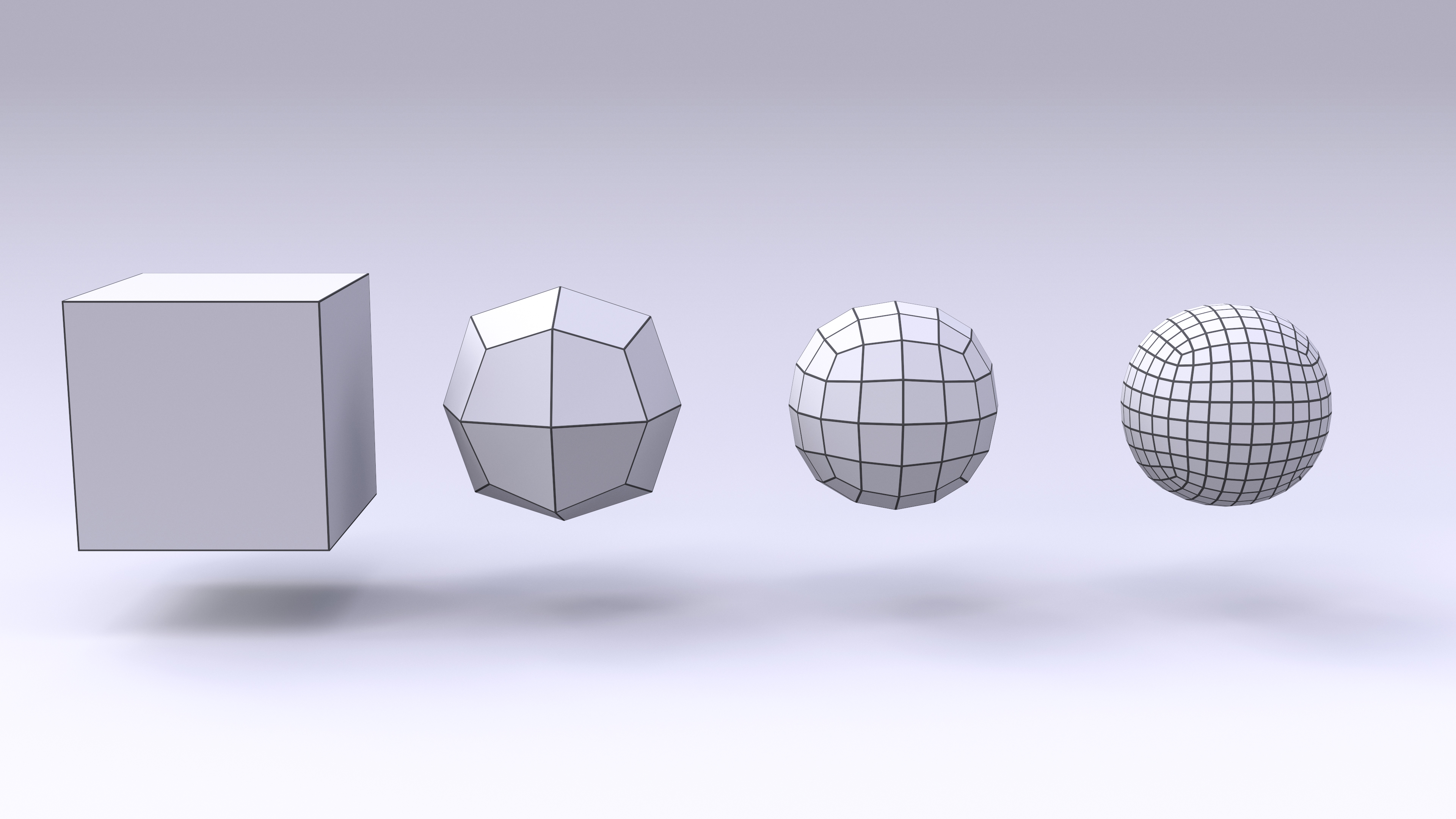
No writing about subdivision surfaces is complete without a picture of a cube being subdivided into a sphere, so Figure 2 shows a render of a cube with subdivision levels 0, 1, 2, and 3, going from left to right. Each subdivided cube is rendered with a procedural wireframe texture that I implemented to help visualize what was going on with subdivision.

Each subdivided mesh is placed into a new mesh; base meshes that require multiple subdivision levels for multiple different geoms get one new subdivided mesh per subdivision level. After all subdivided meshes are ready, Takua then runs displacement. Displacement is parallelized both by mesh and within each mesh. Also, Takua supports both on-the-fly displacement and fully cached displacement, which can be specified per shader or per geom. If a mesh is marked for full caching, the mesh is fully displaced, stored as a separate mesh from the undisplaced subdivision mesh, and then a BVH is built for the displaced mesh. If a mesh is marked for on-the-fly displacement, the displacement system calculates each displaced face, then calculates the bounds for that face, and then discards the face. The displaced bounds are then used to build a tight BVH for the displaced mesh without actually having to store the displaced mesh itself; instead, just a reference to the undisplaced subdivision mesh has to be kept around. When a ray traverses the BVH for an on-the-fly displacement mesh, each BVH leaf node specifies which triangles on the undisplaced mesh need to be displaced to produce final polys for intersection and then the displaced polys are intersected and discarded again. For the scenes in this post, on-the-fly displacement seems to be about twice as slow as fully cached displacement, which is to be expected, but if the same mesh is displaced multiple different ways, then there are correspondingly large memory savings. After all displacement has been calculated, Takua goes back and analyzes which base meshes and undisplaced subdivision meshes are no longer needed, and frees those meshes to reclaim memory.

I implemented support for both scalar displacement via regular grayscale texture maps, and vector displacement from OpenEXR textures. The ocean render from the start of this post uses vector displacement applied to a single plane. Figure 3 shows another angle of the same vector displaced ocean:

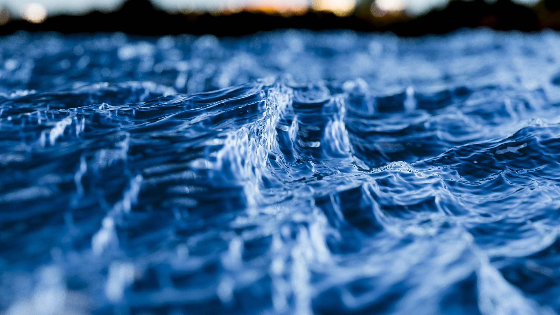
For both ocean renders, the vector displacement OpenEXR texture is borrowed from Autodesk, who generously provide it as part of an article about vector displacement in Arnold. The renders are lit with a skydome using hdri-skies.com’s HDRI Sky 193 texture.

For both scalar and vector displacement, the displacement amount from the displacement texture can be controlled by a single scalar value. Vector displacement maps are assumed to be in a local tangent space; which axis is used as the basis of the tangent space can be specified per displacement map. Figure 4 shows three dirt shaderballs with varying displacement scaling values. The leftmost shaderball has a displacement scale of 0, which effectively disables displacement. The middle shaderball has a displacement scale of 0.5 of the native displacement values in the vector displacement map. The rightmost shaderball has a displacement scale of 1.0, which means just use the native displacement values from the vector displacement map.

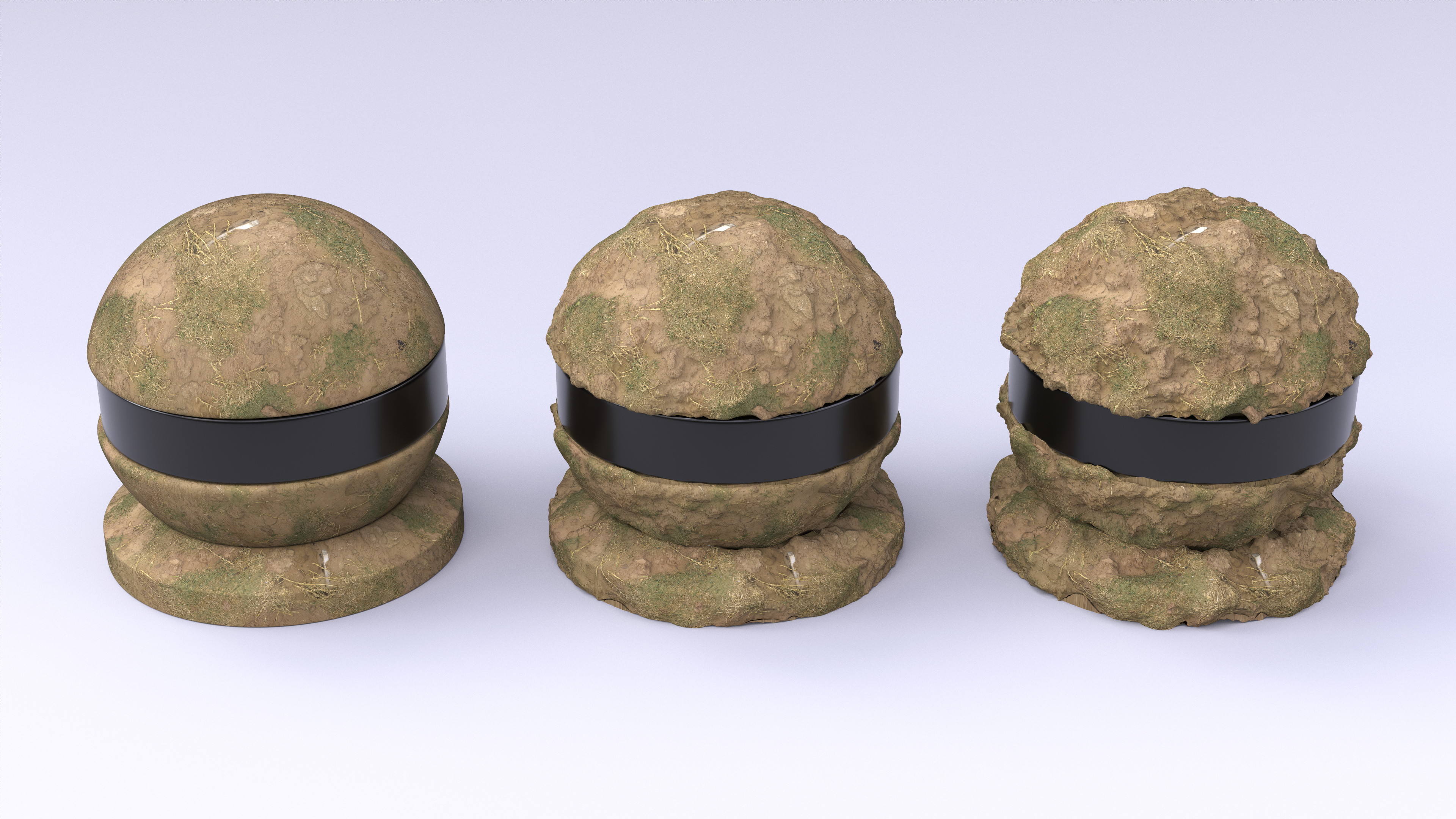
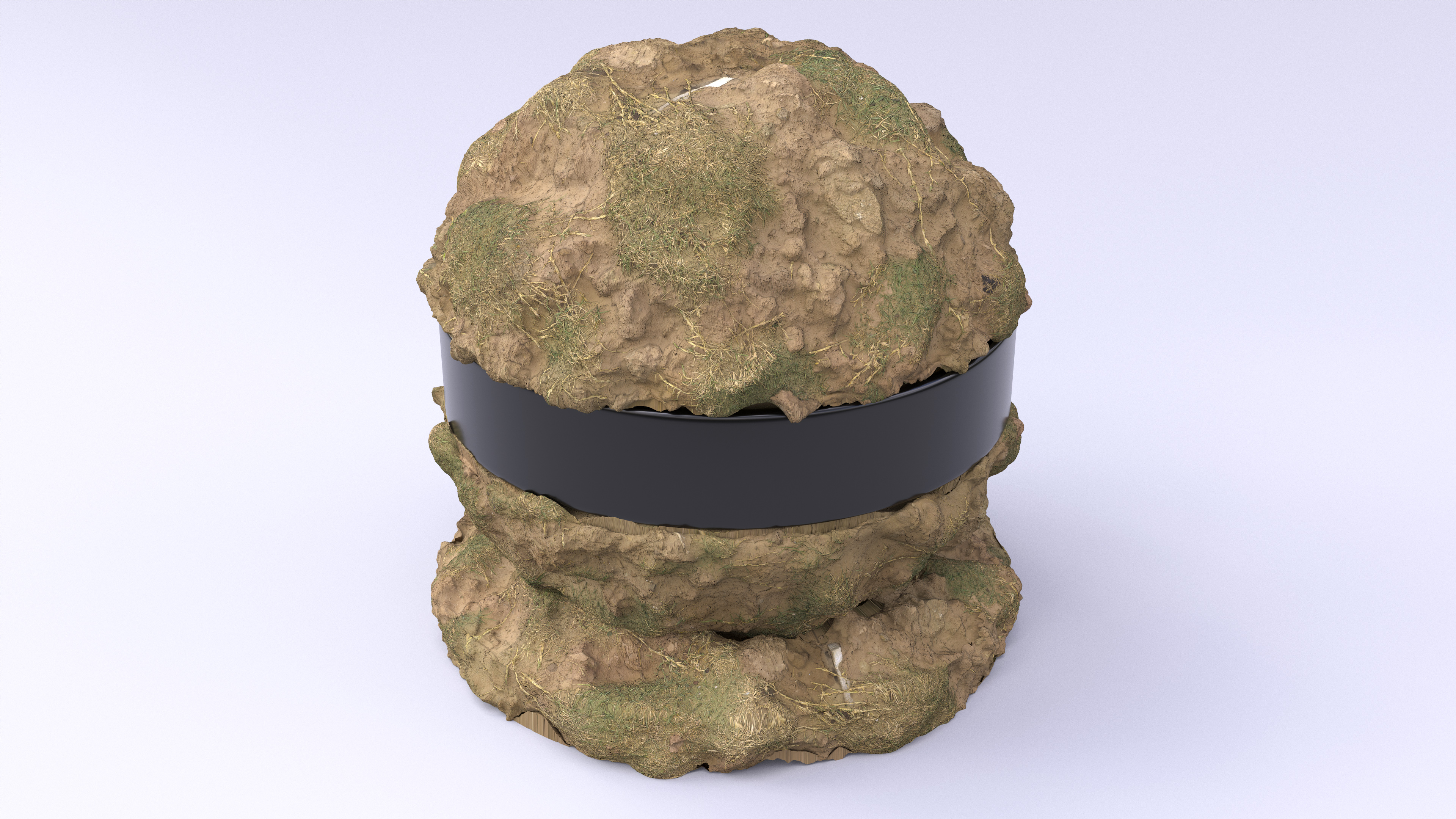
Figure 5 shows a closeup of the rightmost dirt shaderball from Figure 4. The base mesh for the shaderball is relatively low resolution, but through subdivision and displacement, a huge amount of geometric detail can be added in-render. In this case, the shaderball is tessellated to a point where each individual micropolygon is at a subpixel size. The model for the shaderball is based on Bertrand Benoit’s shaderball. The displacement map and other textures for the dirt shaderball are from Quixel’s Megascans library.

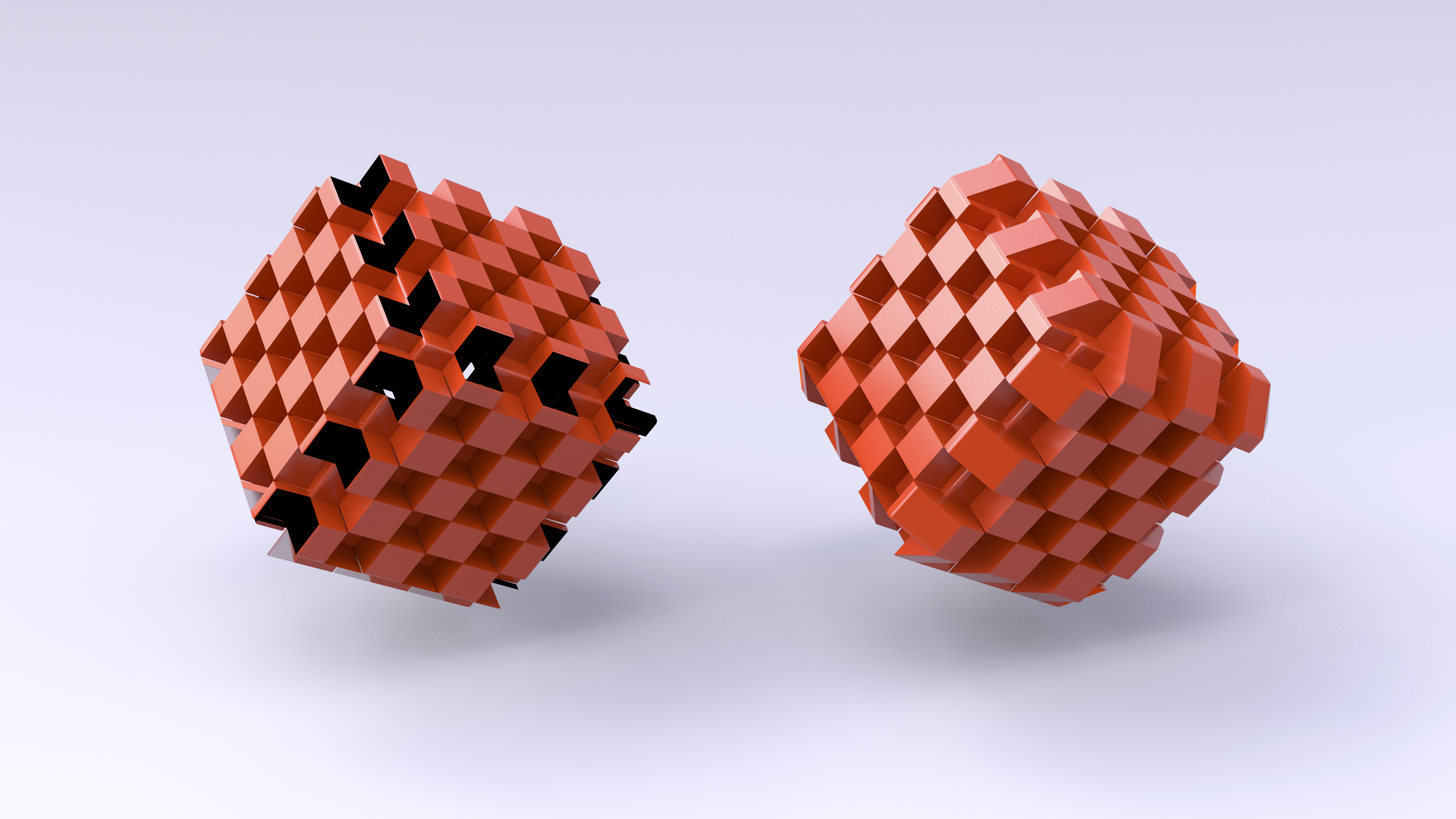
One major challenge with displacement mapping is cracking. Cracking occurs when adjacent polygons displace the same shared vertices different ways for each polygon. This can happen when the normals across a surface aren’t continuous, or if there is a discontinuity in either how the displacement texture is mapped to the surface, or in the displacement texture itself. I implemented an optional, somewhat brute-force solution to displacement cracking. If crack removal is enabled, Takua analyzes the mesh at displacement time and records how many different ways each vertex in the mesh has been displaced by different faces, along with which faces want to displace that vertex. After an initial displacement pass, the crack remover then goes back and for every vertex that is displaced more than one way, all of the displacements are averaged into a single displacement, and all faces that use that vertex are updated to share the same averaged result. This approach requires a fair amount of bookkeeping and pre-analysis of the displaced mesh, but it seems to work well. Figure 6 is a render of two cubes with geometric normals assigned per face. The two cubes are displaced using the same checkerboard displacement pattern, but the cube on the left has crack removal disabled, while the cube on the right has crack removal enabled:

In most cases, the crack removal system seems to work pretty well. However, the system isn’t perfect; sometimes, stretching artifacts can appear, especially with surfaces with a textured base color. This stretching happens because the crack removal system basically stretches micropolygons to cover the crack. This texture stretching can be seen in some parts of the shaderballs in Figures 5, 7, and 8 in this post.

Takua automatically recalculates normals for subdivided/displaced polygons. By default, Takua simply uses the geometric normal as the shading normal for displaced polygons; however, an option exists to calculate smooth normals for the shading normals as well. I chose to use geometric normals as the default with the hope that for subpixel subdivision and displacement, a different shading normal wouldn’t be as necessary.

In the future, I may choose to implement my own subdivision library, and I should probably also put more thought into some kind of proper combined tessellation cache and eviction strategy for better memory efficiency. For now though, everything seems to work well and renders relatively efficiently; the non-ocean renders in this post all have sub-pixel subdivision with millions of polygons and each took several hours to render at 4K (3840x2160) resolution on a machine with dual Intel Xeon X5675 CPUs (12 cores total). The two ocean renders I let run overnight at 1080p resolution; they took longer to converge mostly due to the depth of field. All renders in this post were shaded using a new, vastly improved shading system that I’ll write about at a later point. Takua can now render a lot more complexity than before!

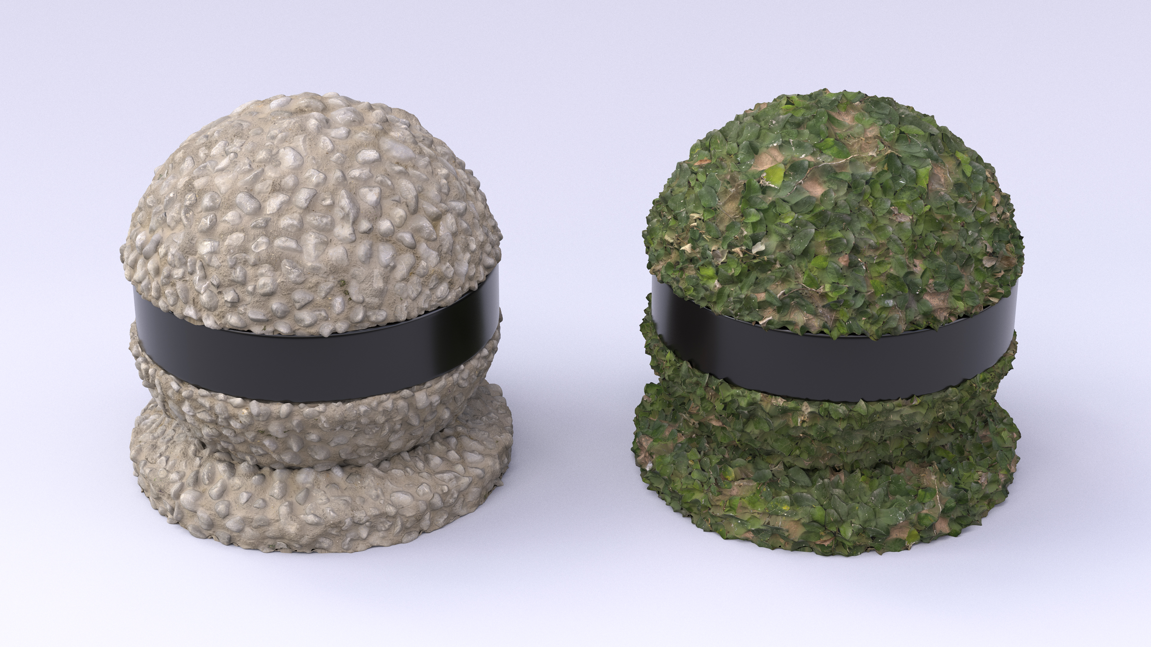
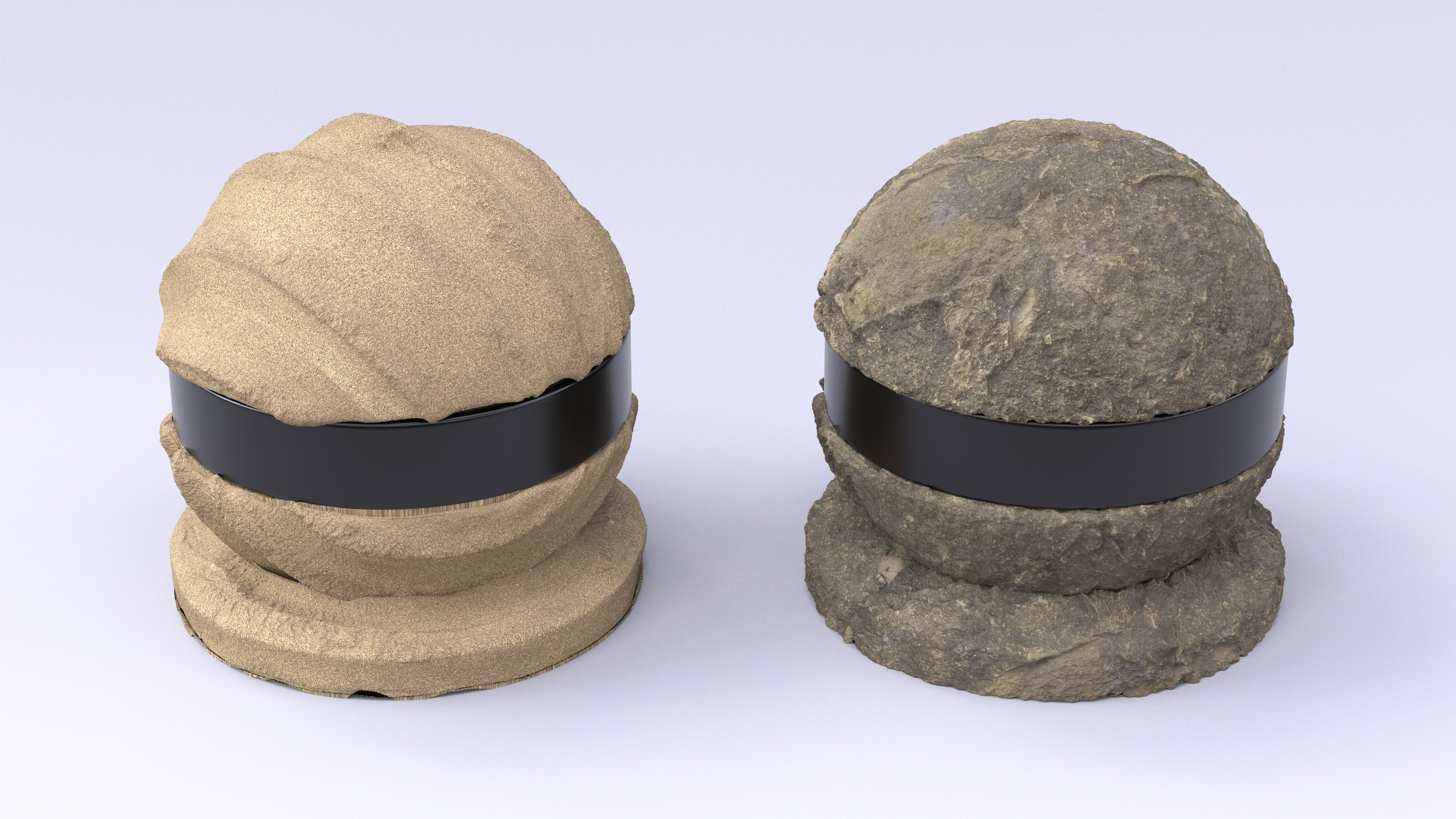
In closing, I rendered a few more shaderballs using various displacement maps from the Megascans library, seen in Figures 7 and 8.

References

Edwin E. Catmull and James H. Clark. 1978. Recursively Generated B-spline Surfaces on Arbitrary Topological Meshes. Computer-Aided Design. 10, 6 (1978), 350-355.

Mark Halstead, Michael Kass, and Tony DeRose. 1993. Efficient, Fair Interpolation using Catmull-Clark Surfaces. In SIGGRAPH 1993: Proceedings of the 20th Annual Conference on Computer Graphics and Interactive Techniques. 35-44.

Johannes Hanika, Alexander Keller, and Hendrik P A Lensch. 2010. Two-Level Ray Tracing with Reordering for Highly Complex Scenes. In GI 2010 (Proceedings of the 2010 Conference on Graphics Interfaces). 145-152.

Takahiro Harada. 2015. Rendering Vector Displacement Mapped Surfaces in a GPU Ray Tracer. In GPU Pro 6. 459-474.

Matthias Nießner, Charles Loop, Mark Meyer, and Tony DeRose. 2012. Feature Adaptive GPU Rendering of Catmull-Clark Subdivision Surfaces. ACM Transactions on Graphics. 31, 1 (2012), 6:1-6:11.

Matt Pharr and Pat Hanrahan. 1996. Geometry Caching for Ray-Tracing Displacement Maps. In Rendering Techniques 1996 (Proceedings of the 7th Eurographics Workshop on Rendering). 31-40.

Brian Smits, Peter Shirley, and Michael M. Stark. 2000. Direct Ray Tracing of Displacement Mapped Triangles. In Rendering Techniques 2000 (Proceedings of the 11th Eurographics Workshop on Rendering). 307-318.